Example 2: Multivariate Regression
RES1 = Intercept1 + 0.1*VAR1 + 0.1*VAR2+ …+ 0.1*VAR100 + E1,
RES2 = Intercept2 + 0.1*VAR1 + 0.1*VAR2 + …+ 0.1*VAR100 + E2, and
RES3 = Intercept3 + 0.1*VAR1 + 0.1*VAR2 + … + 0.1*VAR100 + E3;
where the values for E1, E2, and E3 are random numbers from the normal distribution N(0,0.05).
- Purpose of the Study
- The purpose of this analysis is to examine the effectiveness of the
PLS procedure with this simulated data set and to illustrate how to decide the optimal number of components to retain. Note that since we used N(0,0.05) for an error term for each response variable, we may expect to build a linear model yielding an (average) R-square value of approximately 0.95.
Specifying the Analysis Open the Plssim.sta data file and start General Partial Least Squares Models:
Ribbon bar. Select the Home tab. In the File group, click the Open arrow and select Open Examples to display the Open a STATISTICA Data File dialog box. Open the data file, which is located in the Datasets folder. Then, select the Statistics tab. In the Advanced/Multivariate group, click Advanced Models and from the menu, select General Partial Least Squares to display the Partial Least Squares Models Startup Panel.
Classic menus. From the File menu, select Open Examples to display the Open a STATISTICA Data File dialog box. Open the data file, which is located in the Datasets folder. Then, from the Statistics - Advanced Linear/Nonlinear Models submenu, select General Partial Least Squares Models to display the Partial Least Squares Models Startup Panel.
Select Multiple regression as the Type of analysis, Quick specs dialog as the Specification method, and click the OK button to display the PLS Multiple Regression Quick Specs dialog box.
Click the Variables button to display the standard variable selection dialog box. Select Res1 through Res3 as the Dependent variable list, all of the other variables (Var1 through Var100) as the Predictor variables (covariates), and then click the OK button.
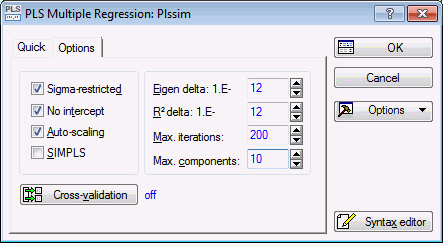
In the PLS Multiple Regression dialog box, select the Options tab. We will extract a maximum of 10 components for this analysis, so enter 10 in the Max components field. The Options tab will now look like this.
We will accept all other defaults, so click the OK button to begin the analysis and display the PLS Results dialog box.
- Reviewing Results Summary
- On the
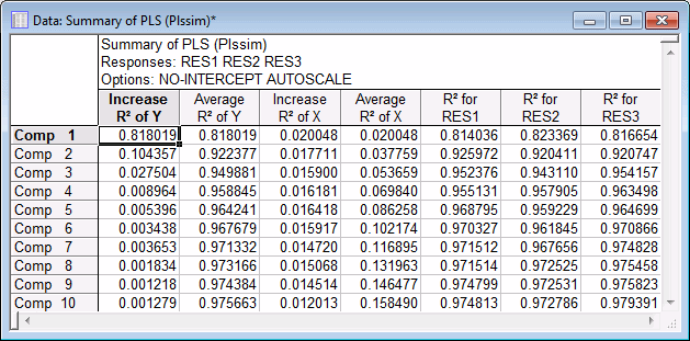
PLS Results dialog box - Summary tab, click the Summary spreadsheet button. The following spreadsheet will be displayed.
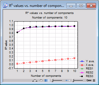
You can visualize these results by clicking the Summary graphics button.
The spreadsheet shows the R-square values and R-square increments for the respective number of components, listed in the rows. The R-square values are computed for the predictor variables (columns in the design matrix; the respective spreadsheet column is labeled R2 of X) and the dependent (response) variable (the respective spreadsheet column is labeled R2 of Y). The average R-square value for the predictor (X) variables is computed as the averaged R-square over the predictor variables (columns in the design matrix); the average R-square value for the Y variables is computed analogously. Also, unlike in STATISTICA General Linear Model (GLM) or Multiple Regression, the R-square values are computed relative to the sums of squared deviations from the origin (0.0) for the centered (de-meaned) predictor variables (columns in the design matrix) and dependent (response) variables.
The plot shows the change in the average R-square values over the number of components. In this plot there appears to be a leveling off of the R-square values for the dependent (response) variables at the point of 2 or 3 components; thus we can select to retain either 2 or 3 components for the final (interpretation of the) results. Three components will explain approximately 95% of the variability in the dependent variables, which is the magnitude of the average R-square value that we expected, given the manner in which the data were generated.
- Regression Coefficients by Number of Components
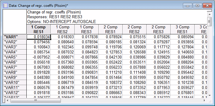
- On the Summary tab, in the Regr. coeffs. by number of coefficients group box, click the Table of results button.
Each column of the spreadsheet shows the regression coefficients for each component and for each response variable.
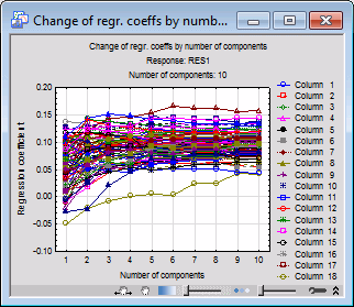
To produce a graphical summary of these results, on the Summary tab, in the Regr. coeffs. by number of coefficients group box, click the Plot button; by default the regression coefficients (versus the number of components) for dependent (response) variable Res1 will be shown.
- Weights for X
- Enter 3 in the Number of components field and click the Weights for X spreadsheet button.
It appears that there are fewer weights for Component 1 with negative values, thus, this component may represent the weights for the global mean of the predictor variables, which were set to (exactly) 0.1 for the computation of the dependent (response) variables.
See also, PLS - Index.

