Example 8.2: Designing and Analyzing a Mixture Experiment with Pseudo-Components

Cornell (1990a, page 41) discusses an experiment involving three ingredients that are used to form bleach for removing grease stains: Bromine, Powder, and diluted HCl. The minimum proportions of each component that must be present in each blend are:

Bromine: L1 = .30 <= x1

Powder: L2 = .25 <= x2

HCl: L3 = .02 <= x3

Thus, the minimum factor setting for each component is constrained by a lower bound (Li). Lower-bound constraints on mixture variables are discussed in the Introductory Overview. The general problem is that the standard simplex-lattice and simplex centroid designs can no longer be constructed. Instead, the designs are constructed for pseudo-components, which are computed as transformations of values for the original factors.

Designing the experiment

Start Experimental Design (DOE).

Ribbon bar. Select the Statistics tab, and in the Industrial Statistics group, click DOE to display the Design & Analysis of Experiments dialog box.

Classic menus. On the Statistics - Industrial Statistics & Six Sigma submenu, select Experimental Design (DOE) to display the Design & Analysis of Experiments dialog box.

On the Advanced tab, select Mixture designs and triangular surfaces.

Click OK to display the Design & Analysis of Mixture Experiments dialog box. Ensure that the Design experiment tab is selected.

The different standard designs for mixture variables are discussed in detail in the Introductory Overview.

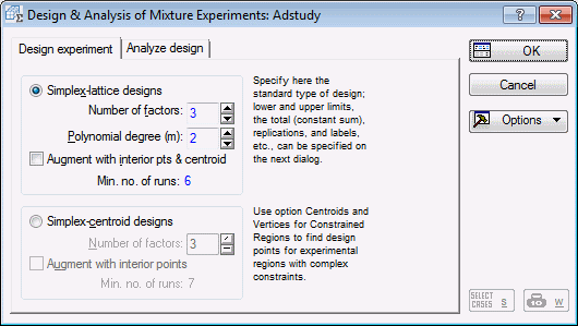
The design described by Cornell (1990a, Table 11) is a {3,2} simplex-lattice design. Thus, ensure that the Simplex-lattice designs option button is selected, type 3 into the Number of factors box, and type 2 into the Polynomial degree (m) box (see above).

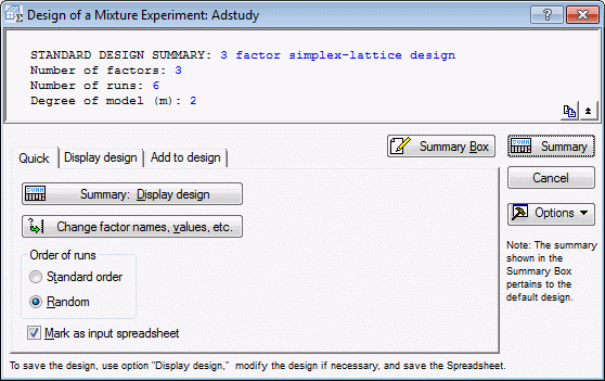
Then, click OK to generate the design and display the Design of a Mixture Experiment dialog box.

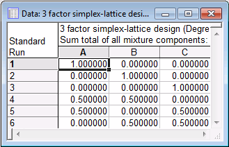
Select the Standard order option button, and click the Summary: Display design button.

This is the same design we used in the previous example. The problem is that the factor settings for all factors span the range from 0 to 1; and 0 is not a valid factor setting for any of the three ingredients in this study.

Introducing lower bounds for factor settings

Click the Change factor names, values, etc. button.

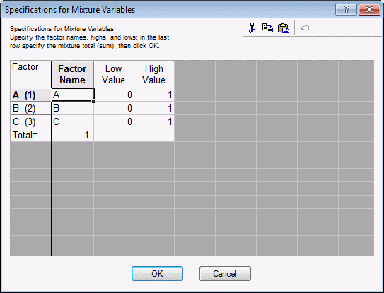
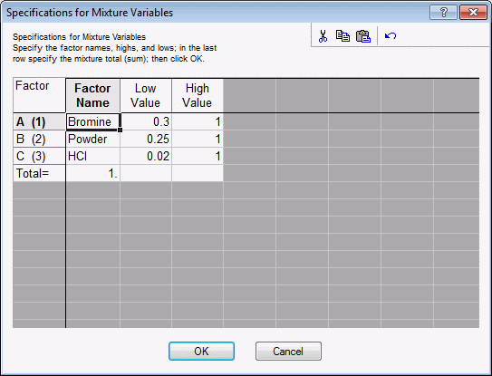
Enter the factor names and the lower bounds for each factor, as shown below (and described in the introduction to this example).

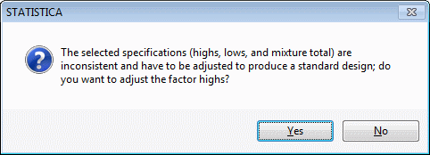
Click OK and the following warning message will be displayed.

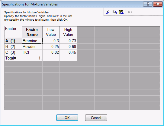
Given the lower bounds, Statistica cannot construct the standard simplex design. Instead, the program will determine the high factor settings, so as to define a sub-triangle inside the full triangular region described by the standard design. Click Yes to see the adjusted high factor settings.

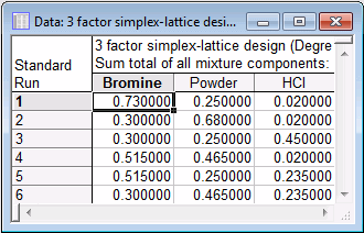
Click OK to accept the adjustment, and then click the Summary: Display design button again to review the design.

Even though it may not be immediately apparent, this design is the same standard simplex-lattice design reviewed earlier, except that it is constructed in a subregion of the original design.

As before, you can save the design in a Statistica data file.

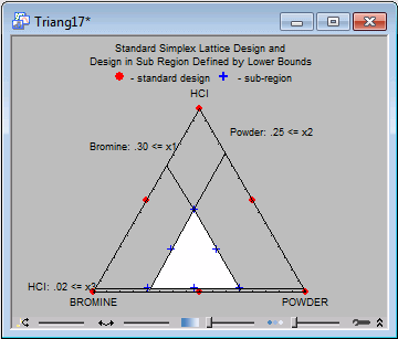
Shown below is a triangular scatterplot of these design points (the original points shown earlier, and adjusted points shown above). (To reproduce this plot, create a file with all design points, and select from the Graphs menu option Stats 3D XYZ Graphs - Ternary graphs; then select a 2D Scatterplot of the design points.)

In this illustration, the lower-bound restrictions for the factors are indicated by lines; those lines define the valid subregion of the full triangle. The standard simplex-lattice design is then constructed within this subregion.

Analyzing the design

Close all spreadsheets/workbooks and analysis dialog boxes.

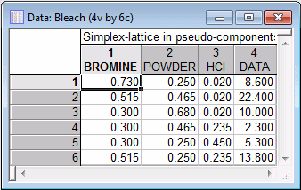
The data from the completed experiment is contained in the example data file Bleach.sta. Open this data file.

Start the Experimental Design (DOE) analysis. In the Startup Panel, select the Advanced tab, and double-click Mixture designs and triangular surfaces to display the Design & Analysis of Mixture Experiments dialog box.

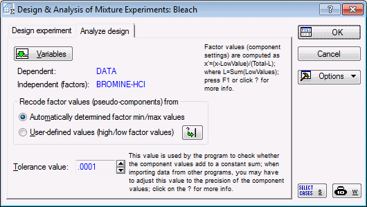
Select the Analyze design tab. Click the Variables button, and in the variable selection dialog box, select Data as the Dependent variable and Bromine, Powder, and HCI as the Independent vars (factors). Click OK.

In the Design & Analysis of Mixture Experiments dialog box, click OK to display the Analysis of a Mixture Experiment dialog box.

Results for pseudo-components

To reiterate (see Introductory Overview, or Example 8.1), the pseudo-component transformation is defined as:

x'i = (xi-Li)/(Total-L)

Here, x'i stands for the i'th pseudo-component, xi stands for the original component value, Li stands for the lower constraint (limit) for the i'th component, and L stands for the sum of all lower constraints (limits) for all components in the design. In effect, this transformation will turn the original component settings into the standard settings for a simplex-lattice design.

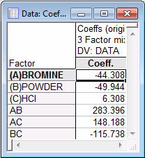
Cornell fits to the data the standard quadratic model; therefore, select the Model tab and select the Quadratic option button. Then, select the Quick tab and click the Summary: Estimates, pseudo components button.

Since there are only six observations in the data file, from which six parameters are estimated, statistical significance tests or standard errors are not available for these estimates.

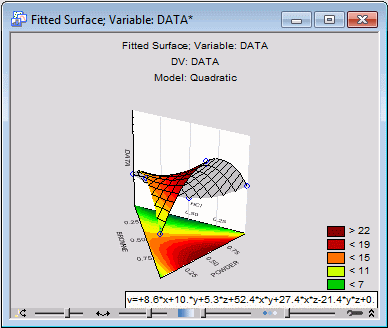
To see the fitted surface, select the Prediction & profiling tab and select the Show fitted function check box. Then, click the Surface plot (fitted response) button.

You can use the Interactive Graphics Controls at the bottom of the graph window to rotate the graph and/or adjust the transparency of the plot areas to view different aspects of the plot.

As in the previous example (Example 8.1), let's also look at the trace plot. After clicking the Trace plot of expected responses button, Statistica will prompt for the reference blend values by displaying the Values for Reference Blend dialog box; the values should be chosen with reference to the original components, not the pseudo-components. Simply accept the default values, and click OK.

Clearly, the less HCl, the larger the dependent variable values. In fact, looking back at the contour plot, it appears that the highest response can be expected when HCl is at its minimum and the other two components are present in about equal proportions, with regard to the pseudo-components (as plotted in the surface).

Results for original components

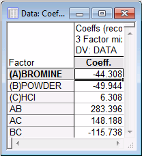
Let's now look at the results for the untransformed raw components. Select the Quick tab, and click the Estimates, original comps button.

Note: you can produce the same results as shown above by performing the standard analysis and suppressing the pseudo-component transformation.

To illustrate, click Cancel in the Analysis of a Mixture Experiment dialog box to return to the Design & Analysis of Mixture Experiments dialog box.

Select the User-defined values (high/low factor values) option button, which displays the Specifications for Mixture Variables dialog box (Statistica will remember the variable selections from the previous analysis).

In this spreadsheet, you can specify the Low and High factor values for the mixture components. (By default the program determines those values from the data). The Low values will be used for the transformation of the raw component settings to pseudo-components. When you now click OK, Statistica will accept 0 (zero) as the minimum for all factors, and, hence, the pseudo-component transformation will not change the factor values (see the transformation described earlier in this example; see also Introductory Overview). Click OK.

Click OK  in the Design & Analysis of Mixture Experiments dialog box to display the Analysis of a Mixture Experiment dialog box.

As you can see, the Estimates, original comps button is not available now (it is dimmed). Since all factor Lows were equal to 0 (zero), the pseudo-component transformation actually did not change the factor values.

Now, on the Model tab, select the Quadratic option button again, and on the Quick tab, click the Summary: Estimates, pseudo-components button to produce the spreadsheet with the coefficients.

As you can see, they are identical to those shown earlier.

Response surface for raw components

Now click the Surface plot (fitted response) button to produce the response surface for the untransformed components.

As you can see, the pseudo-component transformation shown in the earlier graph produced a surface with a much better "resolution," that is, the respective triangular graph only shows the response surface in the valid region (given the lower constraints on the components). Yet, because the pseudo-component transformation is a linear transformation of the factor values, the nature of the response surface has not changed, and, hence, the conclusions from this study have not changed.

See also, Experimental Design.