Example 8.1: Designing and Analyzing a Mixture Experiment

Cornell (1990a) discusses a simple but typical mixture experiment concerned with the average texture of fish patties. Sandwich patties were made of blends of three types of fish: Mullet, Sheepshead, and Croaker. The dependent variable of interest was Texture, as measured by the force (in grams * 10-3) required to puncture the patty surface. We will first design the experiment as reported by Cornell (1990a, page 9), and then analyze the completed experiment.

Designing the experiment

Open the Fish.sta data file and start Experimental Design (DOE).

Ribbon bar. Select the Home tab. In the File group, click the Open arrow and from the menu, select Open Examples to display the Open a Statistica Data File dialog box. Double-click the Datasets folder, and open the Fish.sta data set. Then, select the Statistics tab, and in the Industrial Statistics group, click DOE to display the Design & Analysis of Experiments dialog box.

Classic menus. On the File menu, select Open Examples  to display the Open a Statistica Data File dialog box. The Fish.sta data file is located in the Datasets folder. Then, on the Statistics - Industrial Statistics & Six Sigma submenu, select Experimental Design (DOE) to display the Design & Analysis of Experiments dialog box.

Select the Advanced tab, select Mixture designs and triangular surfaces, and click OK to display the Design & Analysis of Mixture Experiments dialog box.

There are two typical types of experimental designs that are used with mixture variables: Simplex-lattice designs and Simplex-centroid designs; the difference between these designs is explained in the Introductory Overview. In both types of designs, you choose the pure blends representing the corners of the simplex (or triangle, in the case of a three-factor design); the difference between the designs pertains to the choice of the other points in the design.

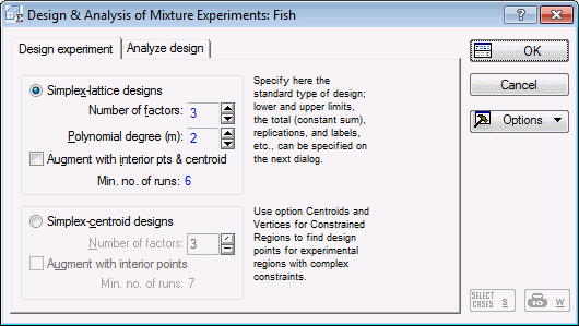
To produce the design for this example study, select the Simplex-lattice designs option button, enter 3 in the Number of factors box, and enter 2 in the Polynomial degree (m) box. The polynomial degree refers to the types of terms in the model that you expect to fit to the mixture data. Clearly, if you want to fit a quadratic model to the data, you need to vary each component in the mixture over at least 3 levels; to fit a cubic model, you need to vary each component in the mixture over at least 4 levels.

The design you have now selected is also referred to as a {3,2} simplex-lattice design (3 factors, polynomial degree of 2).

Reviewing the design

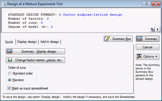
Click the OK button to display the Design of a Mixture Experiment dialog box.

The options in this dialog box are very similar to those described in the other examples, for example, in the context of reviewing 2(k-p) or 3(k-p) designs. To review the current design, click the Summary: Display design button.

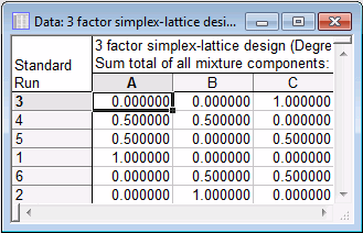
It is apparent that the current design consists simply of the pure blends and two-factor mixtures of the two types of fish.

Factor highs and lows

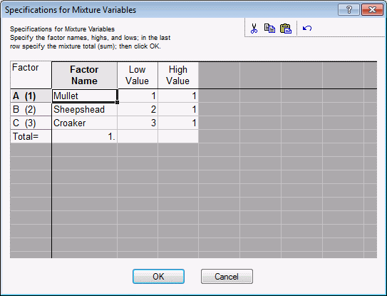
In the Design of a Mixture Experiment dialog box, click the Change factor names, values, etc. button to display the Specifications for Mixture Variables dialog box.

As described, for example, in the context of 2(k-p) designs, you can enter into this dialog box the respective factor names and low and high settings. However, as described in the Introductory Overview, there is an additional constraint. Namely, the sum of all components for each blend must be constant (e.g., the proportions of fish must sum to 100% for each patty). Therefore, in order to maintain a simplex-lattice design as shown above, you cannot enter any arbitrary numbers for the factor highs and lows or for the Total.

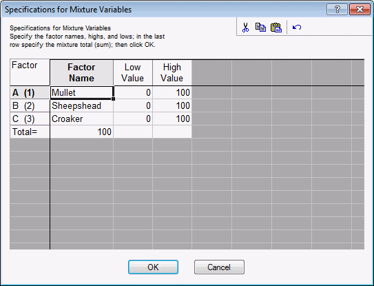
For example, enter the following numbers for the factor highs and lows.

Now click OK, and you will see the following message.

Finalizing and Saving the Design

However, for the current design no special lower constraints are placed on the factors, and the design can be constructed in the full triangular space.

Let's scale the factors in terms of percentages (rather than proportions), and adjust the factor total accordingly (i.e., set it to 100). Enter in the following values.

Click OK to return to the Design of a Mixture Experiment dialog box.

The final design discussed by Cornell (1990a) is a complete replication of the {3,2} simplex-lattice design, that is, two measurements were taken at each point in the design. Therefore, on the Add to design tab, enter 1 into the Number of genuine replicates box and enter 1 into the Number of blank column (dep. vars) box. On the Quick tab, click the Summary: Display design button (the spreadsheet shown below is in Random order, so it will not be in the same order as your results).

This is the final design; you can save it as a standard Statistica data file.

Analyzing the experiment

We will continue using the data file Fish.sta.

Click Cancel in the Design of a Mixture Experiment dialog box to return to the Design & Analysis of Mixture Experiments dialog box.

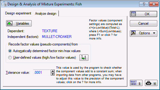
Select the Analyze design tab, and click the Variables button.

In the variable selection dialog box, select Texture as the Dependent variable and Mullet, Sheepshd, and Croaker as the Independent vars (factors). Click OK.

Factor min/max values

The options in the Recode factor values (pseudo-components) from group box pertain to how Statistica will recode the factor values for the final analysis. Specifically, the program will, by default, transform the factor settings into so-called pseudo-components (note that the results for the untransformed factor settings will also be available in the results dialog box).

x'i = (xi-Li)/(Total-L)

Here, x'i stands for the i'th pseudo-component, xi stands for the original component value, Li stands for the lower constraint (limit) for the i'th component, and L stands for the sum of all lower constraints (limits) for all components in the design.

This transformation is also described in the Introductory Overview; see also Cornell, 1990a, Chapter 3.

In short, if there are lower-bound restrictions on the factors, but the design was constructed as a standard simplex-lattice or simplex-centroid design, the factors settings will be rescaled so that the final results can be reviewed and interpreted in terms of the standard simplex design (e.g., triangular graph).

The options in the Recode factor values (pseudo-components) from group box enable you to use the actual factor minima for this transformation (in place of Li), or you can specify User-defined values (high/low factor values).

Tolerance value

The Tolerance value in this dialog box is not to be confused with the tolerance value as discussed, for example, in Multiple Regression. It simply pertains to the "check" for the correctness of the factor settings, that is, whether for all runs the sum of the factor settings is constant.

In particular, when you enter data by hand, it often happens that you may enter .333 to indicate 1/3. Of course, .333 is only accurate for the first 3 digits; to enter the value precisely you would have to enter an infinite series of 3s past the decimal point.

Statistica will perform the check for a constant sum, plus or minus the tolerance value. However, note that the program will always proportionately adjust the factor values so that they sum to the respective constant exactly. Thus, if in a 3-factor experiment where the mixture total is equal to 1, you entered the values .33, .33, .33, the program would adjust those values to .3333333... for each factor.

Reviewing Results

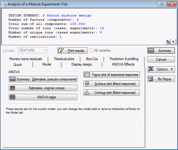
For the current example data file, no additional selections need to be made in this dialog box; simply click OK to display the results dialog box, Analysis of a Mixture Experiment.

If you have read through the examples for 2 and 3-level factorial designs at the beginning of the Examples section, most of the options in this dialog box will be familiar.

In general, you want to fit a model to the data that sufficiently explains the pattern of measurements for the dependent variable. The standard models for mixture designs, as listed on the Model tab, are described in detail in the Introductory Overview. For the current data set, we designed the study for a polynomial model of degree 2, that is, the model of maximum complexity that can be fit is the quadratic model. In its so-called canonical form, the quadratic model for 3 mixture variables can be written as:

ypred = b1*x1+b2*x2+b3*x3

       +b12*x1*x2+b13*x1*x3+b23*x2*x3

Here bi stands for the coefficients, and xi stands for the factor values.

Reviewing coefficients

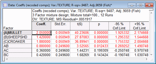
To review the coefficients for the quadratic model, select the Model tab, and select the Quadratic option button. Then, select the Quick tab and click the Summary: estimates, pseudo-components button.

These are the coefficients that pertain to the rescaled factor values, that is, in this case, to the proportions (from 0 to 1) and not the percentage values (from 0 to 100). Remember that the significance tests for the linear factor effects are not independent of each other, and they should be interpreted with caution (since the values for the 3 components must sum a constant total, there are only 2 degrees of freedom for all linear factor effects; see also ANOVA Results below).

From the results displayed in the spreadsheet shown above, it appears that the Mullet by Sheepshd (AB) interaction is statistically significant, and should be included in the model.

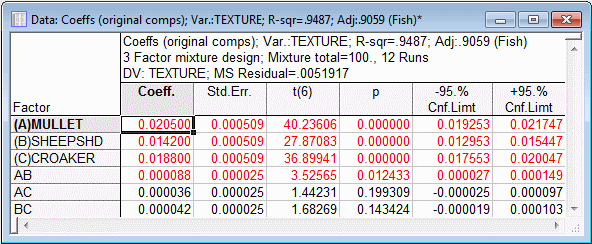
Let's now look at the coefficients for the original, untransformed, components by clicking the Estimates, original comps button. In this case, the transformation only involved dividing the factor values by 100 (to scale them to the range from 0 to 1). Thus the results in this case should be very similar to those reviewed above, except for the magnitudes of coefficients.

As you can see, the coefficients for the original components differ only in their order of magnitude.

ANOVA table

Let's now review the ANOVA table by clicking the ANOVA table button. Two spreadsheets will be produced. The first summarizes the statistical significance tests for models of increasing complexity (i.e., with increasingly more parameters).

The linear model is statistically significant, that is, it fits the data better than the model where all parameters are equal to 0 (zero). Note that the test for the linear parameters has only 2 degrees of freedom, even though the previous spreadsheets showed 3 parameters. To reiterate, since the sum of the mixture components must be constant, the 3 parameters for the simple linear effects only have 2 degrees of freedom associated with them.

Also shown in this spreadsheet are the R² values and the Adjusted R² values. These can be interpreted as in Multiple Regression: R² is the proportion of variance accounted for by the respective model, in the measurements of the dependent variable. The Adjusted R² applies to the R² value an adjustment for the number of terms in the respective model.

Note: proportion-of-variance-accounted-for in this context refers to the variability of the predicted dependent variable values around the respective mean, not 0 (zero). (Some older multiple regression programs sometimes report R² for models without intercept as the proportion of variability around the origin; in the Multiple Regression module, both statistics are reported.)

The most important thing to look at in this spreadsheet is the incremental improvement in fit when additional parameters are added, that is, as more complex models are fitted. In this example, the quadratic model provides an improvement over the linear model, that is almost statistically significant (p=.0507). Thus, we should probably consider at least some second-order effects for inclusion in the final model.

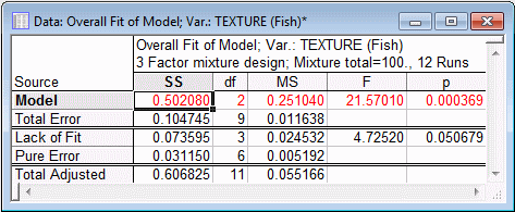
The second spreadsheet shows an overall test for all parameters in the current model.

As you can see, overall, the combined test of all parameters in the quadratic model is highly statistically significant.

Note: the Lack of Fit test cannot be computed for this design. This is because the quadratic model exhausts all information that can be estimated from this second-degree simplex-lattice design. If, for example, you fitted a Linear model by selecting the Linear option button on the Model tab and then clicking the ANOVA table button, the spreadsheet would look like this:

Now only the linear factor effects are in the model, and the residual lack of fit can be tested; of course, it will be identical to the quadratic effects shown in the spreadsheet earlier, since the residual lack of fit that is not due to pure error is due to the quadratic components. Now change back to a Quadratic fit on the Model tab.

Pareto chart of effects

As described in the previous examples (for factorial and central composite designs), the Pareto chart is an efficient tool for presenting the results regarding which factor effects have the greatest impact on the dependent variable of interest. To produce this plot, click the Pareto chart of effects button on the ANOVA/Effects tab.

This graph shows the standardized coefficients, sorted by their absolute magnitudes. Apparently, the linear factor effects are most important in determining the resultant texture of the fish patties.

Surface and contour plots

We can visualize the relationship between the factors and the dependent variable (i.e., the fitted function) in a triangular graph. These graphs are described in detail in the Introductory Overview.

Select the Prediction & profiling tab, and select the Show fitted function check box so the parameter estimates will be displayed in the graph; then click the Surface plot (fitted response) button. Shown below is the resulting graph, after it was rotated to expose the nature of the surface more clearly.

Use the Interactive Graphics Controls at the bottom of the graph window to rotate the graph and/or adjust the transparency of the plot areas to view different aspects of the plot.

In general, as explained in the Introductory Overview, in the triangular graph, the overall mixture constraint (that all component values must sum to a constant) results in a constrained region that can be represented by a triangle. As you move along one of the sides of the triangle shown in the horizontal plane, the blends of the three components change; however, their sum always remains the same (due to the triangular shape of the plane). The surface shown above indicates that the more Mullet in the blend (patty), the greater the surface Texture. However, this surface is not entirely linear, but exhibits slight curvature. This is, of course, consistent with the parameter estimates (for the pseudo-components) reviewed earlier, as well as the Pareto chart produced earlier.

You can also create a Contour plot by clicking the Contour plot (fitted response) button.

Trace plot

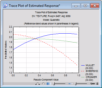
The trace plot provides another view of the triangular surface. Before examining that plot, look at the graph below, which was customized to illustrate how the trace plot is constructed. Specifically, suppose you drew a line from each corner of the triangle to the opposite side. For each point on each line, you can record the predicted value for the dependent variable, or the "altitude" of the response surface over the triangle. Such a trace plot looks like this:

Click the Trace plot of expected responses button. Leave the default settings in the Values for Reference Blend dialog box, and click OK.

Note that, as suggested by the surface, the line for Mullet slopes upward, that is, the greater the relative proportion of Mullet, the greater is the expected value for Texture. The other two lines similarly reflect the bending of the surface.

This plot can be produced for various reference blends, that is, the lines through the triangle do not necessarily have to connect to the opposite side at a right angle, but could be drawn arbitrarily through the triangle. Each such line can be characterized by a reference blend, that is, by a fixed ratio of two components, while the third one varies. Thus, via the Values for Reference Blend dialog box, which is displayed after clicking the Trace plot of expected responses button, you can determine how the trace is to be drawn through the triangle

See also, Experimental Design.