QC Charts Example 10: Specifying Control Charts for Short Production Runs
- Overview
- In some situations the manufacturing process requires short (low-volume) production runs for multiple parts (lots), and each part is characterized by different means and possibly ranges (or standard deviations). Because of the short production runs for each part, allowing only for a small number of samples, meaningful control limits cannot be established for each part. However, you can combine the sample means (and ranges or standard deviations) in a single quality control chart for all parts by applying part-specific transformations to the respective measurements. For example, you could subtract from each measurement the means for the respective parts, thereby, in a sense, placing all measurements on the same scale. (Refer to
Short Run Transformations).
This example demonstrates how to use the Quality Control module in the context of small production runs. It will demonstrate how to transform the original data by subtracting a part-specific constant (the average per lot) from each individual measurement. This will allow you to plot sample statistics of multiple parts (lots) in the same chart.
Let us assume we are manufacturing small lots of surf boards that are painted in three different colors. The paint thickness (in micro meters), which is different for each color, needs to be monitored in an X-bar & R chart. The sample size of 3 is the same for all lots. From past experience we know that the average paint thickness for the different colors is 12.7, 13.6, and 15.0, respectively.
- Setting up the Data File
- Open the data file Shortrun.sta.
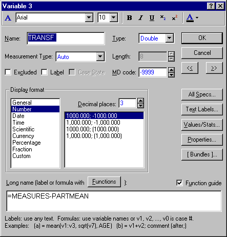
The variable Measures contains the original measurements. The second variable Partmean contains the mean thickness for each color (lot). The third variable Transf contains the transformed values. In particular, the part-specific averages for each color are subtracted from the original measurements, using the following simple spreadsheet formula:
Note: this procedure assumes homogenous variances within lots; if the within-lot variation differs you could use a different transformation (i.e., standardize the data by dividing by part-specific standard deviations). Furthermore, the part-specific average (average per lot) needs to be entered every time you enter an individual measurement (or you can enter those averages ahead of time, and prepare the data file for the new sample measurements), and the Auto-recalculate when data change option for variable Transf should be activated. This option is available by highlighting variable Transf in the data set, clicking the Vars toolbar button, selecting Recalculate Spreadsheet Formulas, and checking the Auto-recalculate when data change check box. - Specifying the Analysis and Reviewing the Chart
- Select Quality Control Charts from the Statistics - Industrial Statistics & Six Sigma submenu or from the Data Mining - Process Optimization - QC Charts submenu to display the
Quality Control Charts Startup Panel. Then select X-bar & R chart for variables on the
Quick tab (or the
Variables tab). Click the
Real-time tab and select the Auto-update option. Now click the OK button to display the
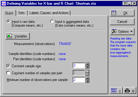
Defining Variables for X-bar & R Chart dialog. On the
Quick tab, click the Variables button and select Transf as the Variable with measurements and click OK. Then specify a Constant sample size of 3.
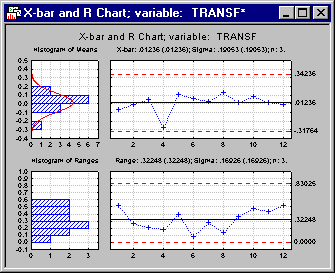
Now click OK to produce the chart.
Apparently, there are no out of control conditions or runs rules violations present. However, when interpreting the chart you should keep in mind that not the original quality characteristic is plotted (paint thickness in micro meter), but the deviations from the part-specific average.
For more information, see Introductory Overview - Short Run Charts. See also QC Chart Examples.


