Example 10.2: Constructing a Design from Vertex and Centroid Points (Example 9.1, Continued)
- Overview
-
Example 9.1 demonstrated the options for finding vertex and centroid points for constrained surfaces (and mixtures). Specifically, those points were computed for a 3-factor design; the low and high settings for each factor were 0 (zero) and 10 respectively, and, in addition, the factor values were constrained by the following two conditions:
(1) xA - 2*xB ≥ 0
(2) xA + xB - xC ≥ 0
Twenty-two vertex and centroid points were computed for these constraints; these points are contained in the example data file Constrr.sta. Open this data file:Ribbon bar. Select the Home tab. In the File group, click the Open arrow and on the menu, select Open Examples to display the Open a Statistica Data File dialog box. Open the Constrr.sta data file, which is located in the Datasets folder.
Classic menus. On the File menu, select Open Examples to display the Open a Statistica Data File dialog box. Open the Constrr.sta data file, which is located in the Datasets folder.
Now, suppose that you want to select from these 22 points the 15 points that can extract the most amount of information about the dependent variable, given a second-order model (i.e., with linear factor main effects, quadratic effects, and two-way interactions).
- Specifying the candidate list and model
- Start the Experimental Design (DOE) analysis:
Ribbon bar. Select the Statistics tab, and in the Industrial Statistics group, click DOE to display the Design & Analysis of Experiments Startup Panel.
Classic menus. On the Statistics - Industrial Statistics & Six Sigma submenu, select Experimental Design (DOE) to display the Design & Analysis of Experiments Startup Panel.
Select the Advanced tab, select D- and A- (T-) optimal algorithmic designs, and click the OK button to display the D- and A- Optimal Designs dialog box.
As before, you need to enter a candidate list of points, that is, the list of points from which you want the program to construct the design.
Click the Variables button, and in the variable selection dialog box, select all three variables in the file. Click the OK button.
Then, select the Model tab.
Select the Lin/quad main eff. + 2-ways option button to specify the second-order model.
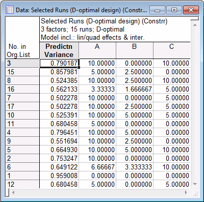
Finally, on the Optimization methods tab, in the Optimization criterion group box, enter 15 into the Number of points in final design box.
Now you are ready to select an optimization method.
- Optimization methods
- The different algorithms for selecting points from the candidate list are described in the Introductory Overview. As a general strategy, it is always a good idea to begin with the fastest and simplest algorithm: Sequential (Dykstra). Actually, unless the candidate list and the number of factors is very large, all methods will typically converge in only a few seconds. Therefore, it is usually a good idea to try different algorithms, perhaps using different starting configurations, to see whether the respective criterion (D or A) was actually optimized, and that the search algorithm did not just get "stuck" in a local minimum.
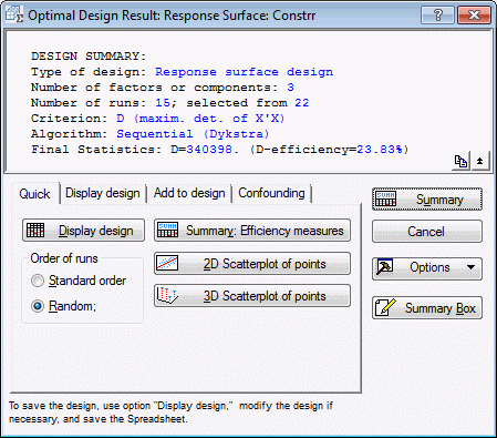
Now, on the Optimization methods tab, click the Sequential (Dykstra) button to display the Optimal Design Result: Response Surface dialog box.
- Reviewing the design
- The options for reviewing the selected design points are very similar to those discussed in the context of other factorial designs (e.g., 2(k-p) designs). To review the final design points click the Display design button.
- Alternative designs
- As mentioned before, it is usually a good idea to try different optimization algorithms with different starting configurations to ensure that one has not selected a solution that is only locally optimal.
Return to the Optimal Design Result: Response Surface dialog box, and click Cancel to return to the D- and A- Optimal Designs dialog box. Then select the Options tab.
Here you have access to various technical parameters of the optimization process. These options are described in detail in the D- and A-Optimal Designs - Options tab topic.
First, in the Initial design group box, select the Select randomly option button. This will cause the program to choose the initial design by random from the candidate list [note that the Sequential (Dykstra) method does not require a design, and for that method, the setting of the options here is disregarded].
Then, click OK and try some of the other optimization techniques.
In most cases, you will get final selections of points that will be very similar to those generated by the Sequential (Dykstra) method; also, the D-efficiency measure will for most random trials be very similar in magnitude. Thus, we can conclude that the first design we reviewed is most likely not only locally optimal, but indeed the best (or close to the best) choice of design, given the candidate list, i.e., given the constrained nature of the experimental region.
Note: in some random trials, you may get the message that the optimization algorithm failed. This can happen when the initial random selection of points produced a very "bad" (i.e., redundant) solution. Simply disregard those messages, and try again, i.e., let the program select another initial design. As an alternative to the random selection, you can also try to use the first n points from the candidate list for the initial design. This is particularly recommended in situations such as the one described in this example, where the first several points represent vertex points of a constrained region. Typically, the vertex points can extract the least redundant information from the experimental region of interest, and therefore, they provide a good start for the optimization algorithms that rely on an initial design (i.e., all algorithms except Sequential (Dykstra)).See also, Experimental Design.