Example 6: X-11 Seasonal Decomposition (Census Method II)
This example is based on a series reporting the monthly US total retail sales from 1953 to 1964. The data set is reported in Shiskin, Young, and Musgrave (1967) to illustrate the results of the X-11 (Census method II) seasonal adjustment procedure. Note that the same example series is used in the Seasonal Decomposition Example; there, the older Census method I seasonal decomposition method was used to analyze this series.
Data File
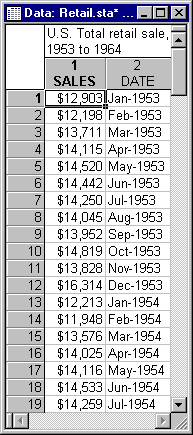
Shown below is a partial listing of the file Retail.sta that contains this series (note that, as reported in Shiskin, Young, and Musgrave, 1967, these numbers are not directly comparable to the official published retail sales figures). Open this data file via the File - Open Examples menu; it is in the Datasets folder.
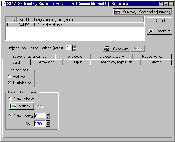
Select Time Series/Forecasting from the Statistics - Advanced Linear/Nonlinear Models menu to display the Time Series Analysis Startup Panel. Click the Variables button to display the standard variable selection dialog. Here, select variable Sales and then click the OK button. Then, click the X11/Y2k (Census 2) - monthly button to display the X11/Y2k Monthly Seasonal Adjustment (Census Method II) dialog.
The options available on this dialog closely follow the options for the US Census Bureau X-11 procedure described by Shiskin, Musgrave, and Young (1967). In general, the X-11 variant of the Census method II is the result of numerous refinements to the simple seasonal adjustment process (e.g., as described in the Introductory Overview for Seasonal Decomposition (Census I); most of these refinements pertain to the treatment of outliers, months with different numbers of trading days, and choices of moving average transformations for isolating the different components. The Introductory Overview discusses those refinements in greater detail.
Determining the Seasonal Model
First plot this series. On the Advanced tab, click the Other transformations & plots button to display the Transformations of Variables dialog. Use the dates recorded in variable Date in the plots, so on the Review & plot tab, click the Dates from a variable option button under Label data points and select the variable Date and then the OK button in the resulting variable selection dialog. Next, select the Scale X axis in plots manually check box and specify Min = 1 and Step = 12. Then, click the Plot button next to the Review highlighted variable button to produce the following plot.
The retail sales show an upward trend and clear seasonal fluctuation. As described in the Introductory Overview, the goal of seasonal decomposition in general is to derive estimates of the seasonal, trend-/cycle, and irregular components that make up the series. The seasonal component can be used to compute a seasonally adjusted series, that is, an estimate of the series after removing seasonal fluctuations.
Additive and multiplicative seasonality
The difference between the additive and multiplicative model is discussed in several places in the Introductory Overview. With regard to retail sales figures, it is conceivable that during the December holiday season, retail sales increase by a relatively fixed amount every year; that is, each year you could add a certain amount to the average sales that year to arrive at an estimate for the December figures. Thus, the seasonal fluctuation would be additive in nature.
Alternatively, each year the sales during December may increase by a factor; for example, they may increase by a factor of 1.3 or 30% over the respective yearly average. In that case, the seasonal fluctuations are multiplicative in nature.
The two types of seasonal fluctuations leave distinctive "signatures" in the series. If the seasonality is additive in nature, the fluctuations are constant around the series, regardless of the overall level of the series. If the seasonality is multiplicative in nature, then the fluctuations are greater when the level of the series is higher. In this example, it rather looks like the seasonality is multiplicative in nature; this would also make more sense intuitively: Most likely, retail sales will increase by a certain percentage each December rather than by a fixed amount. Therefore, click the Cancel button to return to the X11/Y2k Monthly Seasonal Adjustment (Census Method II) dialog and accept the default Multiplicative setting under Seasonal adjust. on the Advanced tab.
Seasonal Decomposition
It is desired to plot later all components that are extracted. STATISTICA will automatically append the seasonal factors, seasonally adjusted series, trend-/cycle, and irregular components to the active work area (refer to Time Series Analysis - Active Work Area for details concerning the memory management in the active work area). Currently (by default), the Number of backups per variable (series) parameter is set to 3. There are four different series that can be appended; thus enter 4 in the Number of backups per variable (series) box.
Start date
The X-11 technique can adjust for months with different numbers of trading days (i.e., Mondays, Tuesdays, etc.). For example, when analyzing the revenues for an amusement park, the number of Saturdays and Sundays in different months will influence greatly the monthly totals. Therefore, the X-11 method requires that you specify a start date for the series (so that the program can then determine the different number of trading days in each month). You may either enter the start month and year into the respective edit fields in the Dates (start of series) box on the Advanced tab, or you can simply take the date from the first observation in the file. For this example, do the latter, that is, click the Variable button under Dates (start of series) box and then select variable Date and the OK button in the resulting variable selection dialog.
Trading day regression
The variability due to trading-day variation (i.e., different numbers of trading days in different months) can be estimated (via least squares regression) from the data. For this example, select to compute the trading-day regression, but only use it to adjust the series if it is statistically significant (as was done in the illustration in Shiskin, Young, and Musgrave, 1967). Thus, select the Compute & adjust conditionally option button on the Trading day regression tab. You may leave all other entries in this box at their defaults (e.g., the Start estimation at year and Adjust beginning at year edit fields will automatically be set to the first observation in the series if no other numbers are entered).
Reviewing result tables
You are now ready to begin the analysis; click the Summary: Seasonal adjustment button. The implementation of the X-11 seasonal adjustment method in the Time Series module follows closely the US Bureau of Census procedure described by Shiskin, Musgrave, and Young (1967). The results consist of a series of spreadsheets and graphs. Shown below are a few selected spreadsheets.
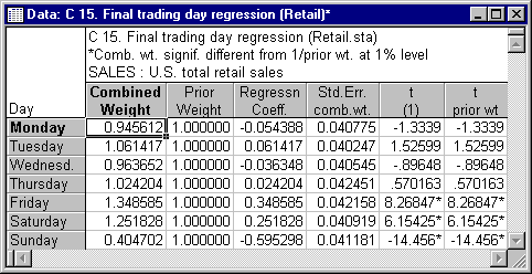
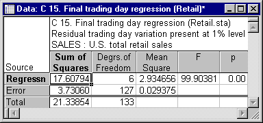
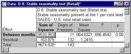
Spreadsheet C 15 Final trading day regression shows that there is highly significant trading-day variation in the series. As expected, the test for stable seasonality is also highly significant; the respective ANOVA table is reported as spreadsheet D 8.
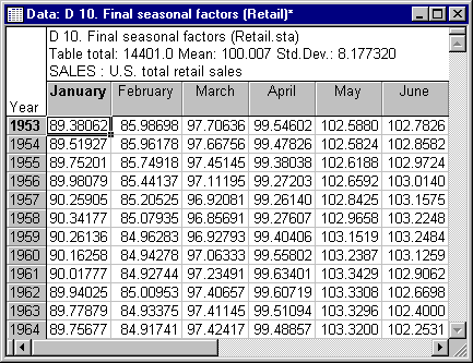
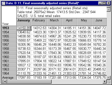
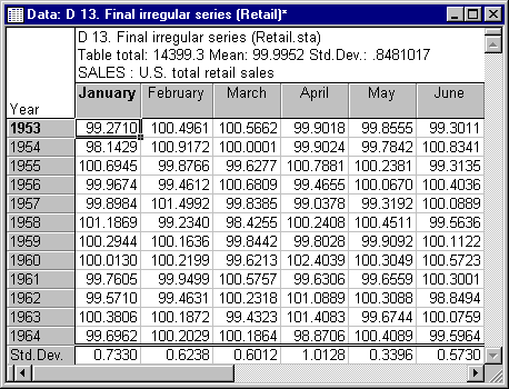
Here are the final estimates of the major components and the seasonally adjusted series. (Note: only the results for the first 6 months of each year are shown).
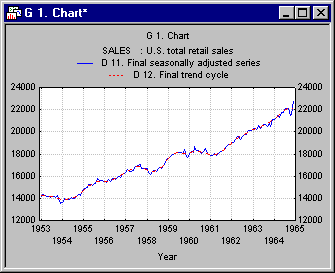
By default, two graphs will also be displayed. The first shows the final trend-/cycle component and the seasonally adjusted series. Clearly, there is only relatively little variability of the adjusted series around the trend/cycle estimate.
The second graph shows different components plotted (categorized) by month.
Return to the X11/Y2k Monthly Seasonal Adjustment (Census Method II) dialog again. The final estimates of the components as well as the final seasonally adjusted series have been added to the active work area.
Finally, look at a summary plot of the original series, the seasonally adjusted series (D 11), and the irregular component (D 13).
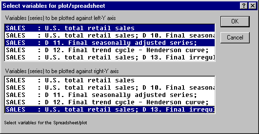
On the Advanced tab, click the Other transformations & plots button to display the Transformations of Variables dialog. Then on the Review & plot tab, click the Plot two var lists with different scales button. In the resulting Select variables for plot/spreadsheet dialog, select the original and seasonally adjusted series for the Variables (series) to be plotted against left-Y axis, and select the Irregular series for the Variables (series) to be plotted against right-Y axis.
Click the OK button to produce the summary plot.
See also, Time Series Analysis Index.

