Example 3: Protein Consumption in Europe
This example illustrates the analysis of a table containing values that are not frequencies. As explained in the Introductory Overview, the results of the correspondence analysis are still valid; however, the total Chi-square value and associated p-value should of course not be interpreted. Remember that correspondence analysis is a descriptive technique used to analyze tables that contain any kind of measure of association, correspondence, similarity, and confusion.
This example is discussed by Greenacre (1984) in the context of the comparison of principal components analysis (see Factor Analysis) with correspondence analysis. For details concerning that comparison, refer to Greenacre (1984, p. 280, Example 9.6). If you are not familiar with the typical results from a correspondence analysis, refer to the Introductory Overview.
The data in the example file Protein.sta represent estimates of the protein consumption from 9 different sources, by inhabitants of 25 countries. Thus, the data are not frequencies, but they are analogous to frequencies in that a total mass of protein is distributed over the cells of the matrix in units of 0.1 gram (per head per day). Following image shows a listing of this datafile. Open this data file using the menu; it is in the Statistica/Examples/Datasets directory.
This example explains analysis of a table containing values that are not frequencies.
Click each process block to know details.

Specifying the analysis
- Select Correspondence Analysis from the Statistics - Multivariate Exploratory Techniques menu to display the Correspondence Analysis (CA): Table Specifications Startup Panel.
- Even though the values in this data file are not frequencies, you can treat them as frequencies. Therefore, on the Correspondence Analysis (CA) tab select the Frequencies w/out grouping vars option button under Input.
- Select the variables. Click the Variables with frequencies button to display the standard variable selection dialog box.
- Select all variables and then click the OK button.
- Click the OK button on the Startup Panel to perform the correspondence analysis. The Correspondence Analysis Results dialog box is displayed.
Reviewing the results
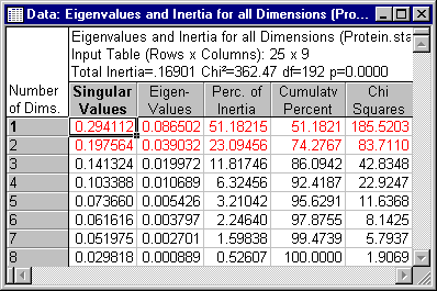
Eigenvalues. To reiterate, the Chi-square value and associated p-value should not be interpreted in this case, since the entries in the table are not frequencies. However, all other results are valid. First click the Eigenvalues button on the Advanced tab.
The total inertia is equal to .16901, and the first two dimensions account for 74.28% of the total inertia. Thus, it appears that the first 2 dimensions account for most of the inertia in this table.
Reviewing the coordinates
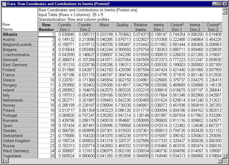
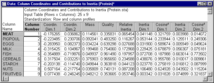
Following image shows the spreadsheets for the row and column coordinates, for the 2-dimensional solution.
- To produce these spreadsheets, click the Row and column coordinates button on the Advanced tab.
- A review of the inertia values for dimension 2 reveals that it is mostly defined by the row point
Portugal and the column point
Fish.
Note: If you refer back to the data file you can see that Portugal has a relatively low protein consumption overall. Greenacre (1984, Table 9.12), therefore, reports the results, treating Portugal as a supplementary point in the analysis. This can easily be accomplished in the Correspondence Analysis module by using the case selection conditions, and excluding the case representing Portugal.
- To do this, click the Cancel button on the Correspondence Analysis Results dialog box to return to the Startup Panel.
- Click the Select Cases button to display the Analysis/Graph Case Selection Conditions dialog box. Here, select the Enable Selection Conditions check box, enter 17 in the or case number field under Exclude cases (from the set of cases defined in the 'Include cases' section), and then click the OK button. Next, click the OK button on the Startup Panel.
- On the Correspondence Analysis Results - Supplementary points tab, click the Add row points button under Supplementary row and/or column points to display the Supplementary Row Points dialog box. Enter the values for Portugal as a supplementary point (example, you can copy the values for Portugal from the data file, and paste them into the spreadsheet.
- Click the OK button to return to the Correspondence Analysis Results dialog box.
If you plot the coordinates for the two-dimensional solution (by clicking the 2D buttons under Plots of coordinates on the Advanced tab), a protein map of the countries emerges, with well-defined regions corresponding to southern Europe, eastern Europe, and northern/central Europe (remember that the study was conducted in the early 70's, so some of the clusters of countries might not seem as homogeneous any more). This pattern becomes defined even more clearly when Portugal is removed from the analysis and only displayed as a supplementary point. The horizontal axis appears to be identified on one end by higher consumption of cereals and nuts (in countries like the former Yugoslavia, Bulgaria, and Rumania), and on the other end by greater consumption of meat and milk; the second axis is characterized on one end by higher consumption of fish (in, for example, Norway, Finland, and Sweden), and on the other end by higher consumption of pork, poultry, and to a lesser extent eggs (in countries like, for example, Austria, the Netherlands, and West Germany).


