Example 3: Frequency Tables

Overview. This example is based on a (fictitious) data set summarizing the results of an opinion survey. Suppose you own several sports bars in your city. In each bar you have two or three big-screen televisions on which you show various sporting events. Because you cannot show all possible sporting events that are simultaneously available on TV, you want to learn in which sports your customers are most interested.

A survey is conducted in which 100 customers (who are randomly chosen at different times in different bars) are asked to express their interest in watching various types of sports on television. Specifically, each respondent is given a list of 14 sports and then asked to indicate their interest in watching the respective sport using a 4-point scale. The four points on that scale are labeled 1) Always interested, 2) Usually interested, 3) Sometimes interested, and 4) Never interested. The Sports.sta data file is a listing of the fourteen sports included in the survey, and is shown below in the Variable Specifications Editor (accessible by selecting the Data tab, and in the Variables group, clicking All Specs).

Data file. The responses were recorded in the example data file Sports.sta. Each variable in that file represents one sport (see above), and each row represents the responses from a single subject. For each sport, the interest expressed by the subjects was recorded on a 4-point scale, and text values were entered to identify the responses.

Open the Sports.sta data file.

Ribbon bar. Select the Home tab. In the File group, click the Open arrow and on the menu, select Open Examples. The Open a Statistica Data File dialog box is displayed. Sports.sta is located in the Datasets folder.

Classic menus. From the File menu, select Open Examples to display the Open a Statistica Data File dialog box; Sports.sta is located in the Datasets folder.

Frequency Tables. You can first look at the interest generated by the more popular sports, that is, football, baseball, and basketball. Start the Basic Statistics and Tables module.

Ribbon bar. Select the Statistics tab. In the Base group, click Basic Statistics to display the Basic Statistics and Tables dialog box.

Classic menus. From the Statistics menu, select Basic Statistics/Tables to display the Basic Statistics and Tables dialog box.

Double-click Frequency tables to display the Frequency Tables dialog box.

Click the Variables button, select the first three variables (Football, Baseball, Basketball), and click the OK button.

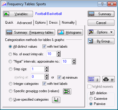
In the Frequency Tables dialog box, select the Advanced tab to see various options related to how the data can be tabulated.

This tab contains many options that will modify the display and categorization of the frequency tables; various tests for normality and graphical ways to visually inspect variables for normality are available on the other tabs. For this example, accept the default categorization method (i.e., All distinct values, with text labels), and click the Summary: Frequency tables button to produce the frequency tables, one for each variable selected.

As you can see in the results spreadsheet for variable Football, 39% of the respondents say they are Always interested in watching football; 16% say they are Usually interested, etc. Overall, 81% of the respondents fall into the categories Always, Usually, and Sometimes interested combined; only 19% say they are Never interested.

Producing histograms. Note that informative histograms of all selected variables can easily be produced by returning to the Frequency Tables dialog box and clicking the Histograms button.

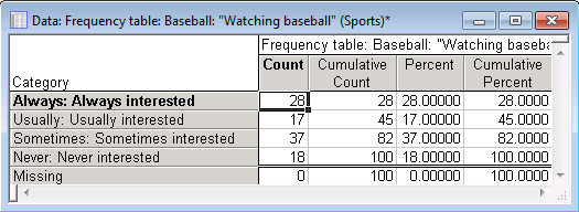
Now look at the results spreadsheet for variable 2 (Baseball).

Here, you can see that the majority of the respondents (37%) are only Sometimes interested in watching baseball. However, 28% of the respondents say they are Always interested.

Graphics options. Practically all of these results can be displayed graphically via the graphics options available in the Results dialog box.

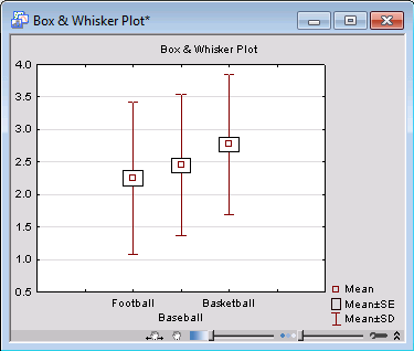
Select the Descr. (descriptive statistics) tab, and click the Box & whisker plot for all variables button. The Box-Whisker Type dialog box is displayed; select the Mean/SE/SD option button as the box-whisker type, and click the OK button to produce the graph.

The variability in responses for each of these variables appears to be similar; however, there seems to be a greater interest in watching football as indicated by the smaller mean response for that variable (remember that 1 indicated greatest interest and 4 indicated the least interest). This can also be seen when you compare the frequency tables for these three variables.

Now look at the 3D Bivariate distribution histogram. When you click the 3D histograms, bivariate distributions button, you are prompted to select the variables for this plot. For this example, select Football in the First variable list, Baseball in the Second variable list, and click the OK button. (Note that if you select more than one variable in a list, several 3D histograms are produced, one for each pair of variables selected.)

From a visual inspection of this bivariate distribution, it appears that there is a correlation between the responses given for variables Football and Baseball. Indeed, if you were to perform a correlation analysis, you would see that there is a Spearman correlation of .6785 between these two variables, which would indicate that subjects who prefer watching football also prefer to watch baseball.

Summary. From this analysis so far, you have learned that, not surprisingly, football and baseball are at the top of the list of spectator sports in the sample. The next question of interest would be to find out what the overlap between sports is. For example, if your clientele consists of a certain percentage of sports "nuts" who would watch any football, baseball, or basketball game, then perhaps you could only show one of those games at a time and reserve your other TV screen for something entirely different, such as tennis or marathons. However, you would first want to know how much of an overlap there is between sports, and which sports would attract an audience that is different from the one that likes to watch football. See Example 4: Stub-and-Banner Tables for further details.

See also, the Basic Statistics and Tables Index and Overviews.