Example 2: A Confirmatory Factor Analysis
Lawley and Maxwell (1971, chapter 7) present techniques for confirmatory factor analysis. These authors are careful to point out that estimation of standard errors must be adjusted when a correlation matrix is analyzed instead of a covariance matrix. They give formulae for computing standard errors when a covariance matrix is analyzed, and provide an alternative method for computing standard errors when the sample correlation matrix is analyzed. The formulae are illustrated with a numerical example, the results of which are presented in their Tables 7.9 (page 99) and 7.10 (page 102).
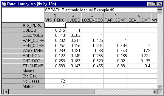
The Lawley-Maxwell example was based on an analysis in a paper by Jöreskog and Lawley (1968), which used data from Holzinger and Swineford (1939). Nine psychological tests were administered to seventh and eighth grade students. The correlation matrix for these data is in the Lawley.sta data file. Open this data file via the File - Open Examples menu; it is in the Datasets/SEPATH folder. Part of this file is shown below.
The tests were (1) Visual Perception, (2) Cubes, (3) Lozenges, (4) Paragraph Comprehension, (5) Sentence Completion, (6) Word Meaning, (7) Addition, (8) Counting Dots, and (9) Straight-curved Capitals. The Lawley-Maxwell example is a typical one, in that each factor is restricted to load on only 3 or 4 manifest variables, and the factors are allowed to correlate with each other. Moreover, by examining what the variables that load on each factor have in common, we can see why the factors are named VISUAL, VERBAL, and SPEED.
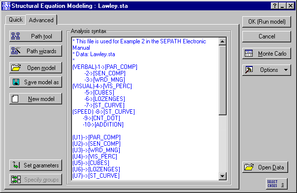
The model is portrayed in the diagram illustration shown below.
The model file corresponding to this diagram is Lawley.cmd. Open this file by clicking the Open model button on the Advanced tab of the Structural Equation Modeling Startup Panel (accessed by selecting Structural Equation Modeling from the Statistics - Advanced Linear/Nonlinear Models submenu) to display a standard Open File dialog and selecting Lawley.cmd in the /Examples/Datasets/SEPATH directory of STATISTICA.
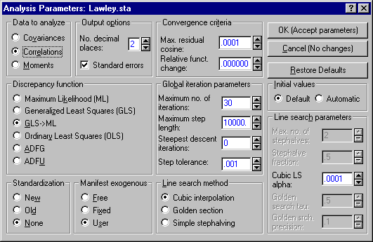
You can reproduce both sets of results in the Lawley and Maxwell tables. First, to simulate what happens with most covariance structure analysis programs, analyze the correlation matrix incorrectly as though it were a covariance matrix: click the Set parameters button on the Advanced tab of the Structural Equation Modeling Startup Panel to display the Analysis Parameters dialog. Under Data to Analyze, select the Covariances option button. Set the number of decimal places to 2 to make the comparison with the Lawley-Maxwell tables easier.
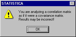
Click the OK (Accept parameters) button in the Analysis Parameters dialog, and then click the OK (Run model) button in the Structural Equation Modeling Startup Panel. Before beginning iteration, STATISTICA will display a warning message indicating that you are about to analyze a correlation matrix (incorrectly) as if it is a covariance matrix.
Click the OK button to proceed with the (incorrect) analysis. You will obtain the erroneous standard errors described by Lawley and Maxwell. Click OK in the Iteration Results dialog, and click the Model summary button on the Structural Equation Modeling Results dialog - Quick tab. (The curious reader might try running this example with other structural modeling programs and comparing the results to those shown below.)
Now, return to the Analysis Parameters dialog, and reset the Data to Analyze to Correlations.
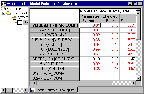
Then re-execute the iteration. You will see estimates and standard errors as shown below.
These standard errors are identical to those reported by Lawley and Maxwell as the correct values, which they obtained by using corrected formulae.
See also, SEPATH Analysis - AutoIndex.

