Support Vector Machine Example 2 - Regression
Support Vector Machine Example 1 is a classification problem, that is, the output was a categorical variable, indicating that the case belongs to one of a number of discrete classes.
STATISTICA SVM can also be used for regression problems, where the output is a continuous numeric variable, in which context it acts as a nonlinear regression technique, where the complexity of the nonlinear regression curve is controlled via the number of support vectors, but of course the designer does not explicitly state a functional form for the regression curve. Hence, it is a nonparametric technique.
- Data file
- Open the Poverty.sta data file, which is located in the /Example/Datasets directory of STATISTICA. The data are based on a comparison of 1960 and 1970 Census figures for a random selection of 30 counties. The names of the counties are entered as case names. This example data file is also discussed in Multiple Regression Example 1: Standard Regression Analysis.
- Starting the analysis
- Select Machine Learning (Bayesian, Support Vectors, Nearest Neighbor) from the Data Mining menu to display the Machine Learning Startup Panel. Select Support Vector Machine and click the OK button to display the Support Vector Machines dialog.
- Analysis settings
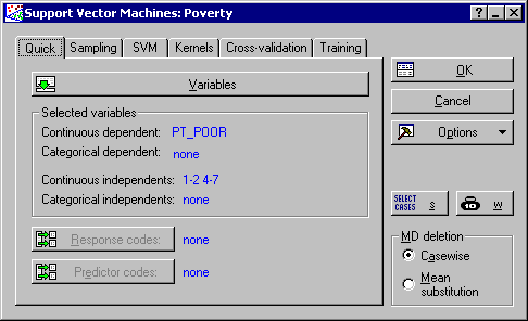
- Click the Variables button to display a standard variable selection dialog, select PT_POOR as the Continuous dependent variable and all of the other variables in the data file as the Continuous predictor (independent) variable list, and click the OK button.
At this stage, you can change the specifications of the analysis, e.g., the sampling technique to be used for dividing the data into train and test samples, the SVM and kernel types, etc. Note that some of these analysis settings are not available until the variables are selected. It is recommended that you always provide a test sample as an independent check on the model performance. The Divide data into train and test samples check box and the Use random sampling option button are selected by default on the Sampling tab.
Note. If your data set is particularly small, the finite data size effect might be large enough, which can render the SVM algorithm from obtaining a good estimate of the model parameters (such as capacity and epsilon). In circumstances such as this, you can resort to the cross-validation method for, generally speaking, obtaining more reliable estimates of these parameters.
One thing you may have noticed by now is the difference between the typical values of the independent variables. This may be counter productive when constructing a good SVM regression model. To alleviate this problem you may want to rescale your variables to lay in the range 0 to 1. This will ensure that all variables are treated on the same scale. To do this, display the Training tab and select the Scale continuous independent variable(s) and Scale continuous dependent variable check boxes.
Leaving the rest of the options at the default settings, click the OK button. This will initiate SVM training (model fitting) which is carried out in two stages. In the first stage, a search is made for estimates of capacity and epsilon that achieve the lowest regression error. In the second phase of training, the estimated value of capacity and epsilon are used to train an SVM model using the entire training sample.
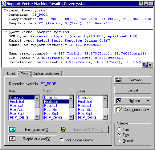
When training is complete, the Support Vector Machine Results dialog is displayed.
- Reviewing results
- From the Results dialog, you can specify to review the results in the form of spreadsheets, reports, and/or graphs.
In the Summary box at the top of the Results dialog are specifications of the SVM model, including the number of support vectors and their types, and the kernels and their parameter(s). Also displayed are other specifications made in the Support Vector Machines dialog, shown here for your reference, including the dependent and independent variable list, and the value of the training constants (capacity, epsilon, and nu). Also listed are the cross-validation results (when applicable) as well as regression statistics for training, test, and overall samples such as mean error squared, standard deviation ratio, and correlation coefficients.
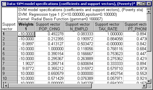
STATISTICA SVM constructs the regression function through a set of support vectors and coefficients. On the Quick tab, click the Model button to display the spreadsheets of these quantities. This can be useful for a detailed review of the SVM model or for inclusion in reports.
Further information can be obtained by clicking the Descriptive statistics button, which will display a spreadsheet containing various regression statistics including the S.D. ratio and the correlation coefficient between the observed and predicted values.
You can also display the spreadsheet of predictions (and include any other variables that might be of interest to you, e.g., independents, residuals, etc., by selecting the respective check box on the Quick tab), as well as create histogram plots of these variables.
Further graphical review of the results can be made by selecting the Plots tab, where you can create two- and three-dimensional plots of the variables and predictions and their residuals. Note that you can display more than one variable in two-dimensional scatterplots.
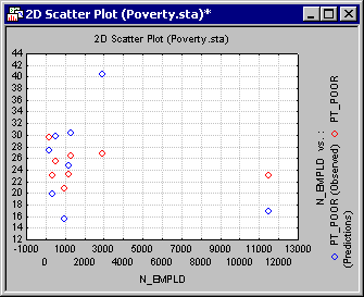
For example, shown above is a scatterplot of the predicted and observed values plotted against the values in variable N_EMPLD. In general, this type of plot will provide an effective way of comparing model predictions with the observed data. To produce the graph shown above, select N_EMPLD from the X-axis list and Observed and Predicted from the Y-axis list. Then click the Graphs of X and Y button.
Note: you can produce these results for any sample by selecting the appropriate option in the Sample group box of the Support Vector Machine Results dialog.Finally, you can perform a "what if?" analysis via the Custom predictions tab. You can define new cases (that are not drawn from the data set) and execute the SVM model. This allows you to perform ad-hoc, "What if?" analyses. The prediction of the model can be created by clicking the Predictions button.


