Example 3: Analyzing a 3³ Full Factorial

Ribbon bar. Select the Home tab. In the File group, click the Open arrow and from the drop-down list select Open Examples to display the Open a Statistica Data File dialog box. Double-click the Datasets folder, and then open the data set.

Classic menus. On the File menu, select Open Examples to display the Open a Statistica Data File dialog box. The data file is located in the Datasets folder.

Shown below is a portion of the data file.

The three factors included in the study were:

In this example, we will first analyze the untransformed dependent variable values to see how the diagnostic plots available in the Experimental Design module enable you to detect the need for transforming the dependent variable values. In general, the purpose of running experiments with factors at more than 2 levels is to be able to detect nonlinearity in the relationships between the factors and the dependent variable of interest. Thus, we will test in this example whether a nonlinear model is necessary to explain the dependent variable values.

Specifying the design. Start the Experimental Design (DOE) analysis:

Ribbon bar. Select the Statistics tab, and in the Industrial Statistics group, click DOE to display the Design & Analysis of Experiments Startup Panel.

Classic menus. On the Statistics - Industrial Statistics & Six Sigma submenu, select Experimental Design (DOE) to display the Design & Analysis of Experiments Startup Panel.

On the Quick tab, select 3(k-p) and Box-Behnken designs and click the OK button.

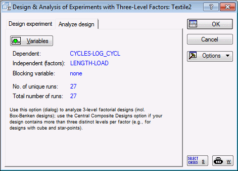
In the Design & Analysis of Experiments with Three-Level Factors dialog box, select the Analyze design tab.

Click the Variables button, and select as the Dependent variables both Cycles and Log_Cycl; select as the Indep (factors) the three variables Length, Amplitud; and Load and click OK.

In the Design & Analysis of Experiments with Three-Level Factors dialog box, click OK to display the Analysis of an Experiment with Three-Level Factors dialog box.

If you reviewed the previous three examples - Example 1.1: Designing and Analyzing a 2(7-4) Fractional Factorial Design, Example 1.2: Analyzing a 26 Full Factorial, and Example 2: Designing and Analyzing a 35-Factor Screening Design - most of the options in this dialog box should be familiar. A new option that requires some explanation is the Use centered & scaled polynomials check box on the Quick tab in the ANOVA group box. This option determines how the model is parameterized.

Centered and uncentered polynomials

Because the factors in this study have 3 levels each, each ANOVA main effect has 2 degrees of freedom, and each (full) interaction has 2 * 2 = 4 degrees of freedom. There are different ways in which we can partition these effects and interactions.

Centered and scaled polynomials

When the Use centered & scaled polynomials check box is selected, Statistica recodes the factor values during computations so that the resulting effect estimates can be interpreted analogously to the two-level case. Specifically, for main effects, the program estimates two parameters:

Original factor setting	Linear Effect	Quadratic Effect
Low (-1)	-1	-2/3
Medium ( 0)	0	4/3
High (+1)	1	-2/3

For balanced standard designs (as produced by the Experimental Design module), this parameterization will result in effect estimates for linear and quadratic effects that can be interpreted in the standard manner, namely that:

1. linear main effects represent the difference between the low and high factor settings for the respective factor, and
2. quadratic main effects represent the difference between the respective medium setting and the average of the low and high settings.

The interactions are scaled and centered accordingly, so that the respective effect estimates can be interpreted as in the 2-level case. The effect estimate for the linear-by-linear interaction between two variables can be interpreted as half the difference between the linear effect of one factor at the low and high settings of the other factor.

The linear-by-quadratic interaction can be interpreted as half the difference between the linear effect of one factor at the medium setting and the average at the low and high settings of the other combined.

The quadratic-by-quadratic interaction can be interpreted as half the difference between the quadratic effect of one factor at the medium setting and the average at the low and high settings of the other combined.

This parameterization will yield ANOVA results that are the same as those you would get if you were to compute the respective sums-of-squares via the General ANOVA/MANOVA module.

Non-centered polynomials

Another parameterization is to simply recode the factor values (xi) to the ±1 range, and then to code the quadratic effects as xi2, the linear interactions as xi*xj, the linear by quadratic interactions as xi*xj2, and the quadratic by quadratic interactions as xi2*xj2. This parameterization is more convenient if we want to use the estimated coefficients for prediction purposes.

Results for untransformed dependent variable

The parameter estimates reported in Box and Draper (1987, page 208) pertain to the simple linear equation for the coded variables; therefore, clear the Use centered & scaled polynomials check box.

Then, click on the Model tab, and select the 2-way interactions (linear, quadr) option button in the Include in model group box.

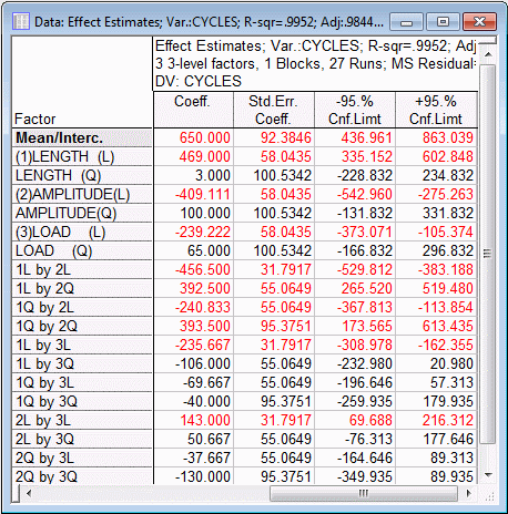
Select the Quick tab, and click the Summary: Effects estimates button in the ANOVA group box. A message is displayed concerning the center/scale polynomial effects. Click the OK button in the message.

Shown above are the 4 right-most columns of the spreadsheet, with the coefficients for the recoded (±1) factor values. A quick check of the column of t-values (not shown in the illustration above) reveals, among several lower-order effects, a strong Length (linear) by Amplitude (quadratic) interaction, and Length (quadratic) by Amplitude (quadratic) interaction.

Response surface

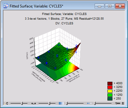
Analysis of an Experiment with Three-Level Factors dialog box, and on the Quick tab, click the Surface plot of fitted response button in the Predicted (estimated) response group box.

In the Select factors for 3D plot dialog box, specify to plot the fitted surface for the Length and Amplitude factors. Click OK.

In the Select factor values dialog box, accept the default mean value (45) for the third factor, and click OK to produce the graph.

This surface shows a strong upward bend toward the upper-right corner. Perhaps, by rescaling the dependent variable Cycles so that very large values are "pulled in," you could change this surface into an almost linear plane, that is, you could drop the complex interaction.

Note: you can use the Interactive Graphics Controls at the bottom of the graph window to adjust the plot areas transparency and to scroll and pan in order to interactively scale the graph.

Observed vs. predicted values

Select the Prediction & profiling tab, and click the Predicted vs. observed values button to produce the graph. Note that the surface plot could have been produced from this tab also.

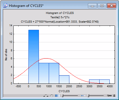
It appears that the values are "bunched together" at the low end of the scales. Again, it seems that the data could be transformed, to pull in the high values for the Cycles variable. This conclusion also seems to be supported if you produce a simple histogram of the variable Cycles from the Statistica Graphs tab (ribbon bar) or from the 2D Graphs menu (classic menus).

Box-Cox procedure

Select the Box-Cox tab and click the Box-Cox Transformation button to find an appropriate transformation for the dependent variable using the Box-Cox procedure (Box and Cox, 1964; see also Gunst, Mason, and Hess, 1989; Snee, 1986).

Reviewing results for the transformed dependent variable

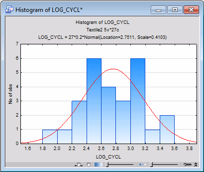
Shown below is the histogram for the log10-transformed dependent variable Log_Cycl, which you can produce from the Statistica Graphs tab (ribbon bar) or from the 2D Graphs menu (classic menus).

While not perfectly normal, the distribution now looks a lot more symmetrical.

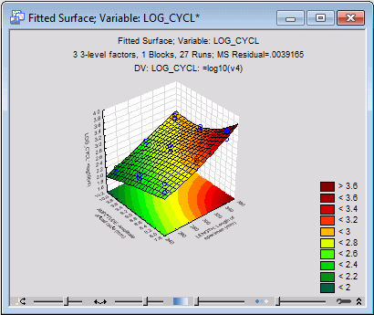
Now, in the Analysis of an Experiment with Three-Level Factors dialog box, change the variable in the Variable box to log_cycle and click the Surface plot of fitted response button either on the Quick tab or the Prediction & Profiling tab to produce at the fitted 3D surface for the transformed dependent variable, for variables Length and Amplitude (setting variable Load at its mean: 45).

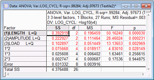
Now the surface looks more like a linear plane, and, if you review the ANOVA table, you will see that the Length (quadratic) by Amplitude (quadratic) interaction is no longer statistically significant

However, the linear-by-quadratic interaction still is statistically significant.

Select the ANOVA/Effects tab (or the Quick tab) and click the ANOVA table button. As you can see, the Length by Amplitude interaction (linear and quadratic combined, with 4 degrees of freedom) is statistically significant.

Box and Draper (1987) accept as the best sufficient model for the transformed dependent variable, the simple linear-main-effects-only model.

On the Quick tab, click the Means plot button in the Observed marginal means group box.

In the Compute marginal means for dialog box, select Length and Amplitude as the Factors, and click OK.

In the Arrangement of Factors dialog box, select Length as the x-axis, upper and Amplitude as the Line pattern. Click OK.

It appears that the interaction is entirely due to one mean.

Specifically, the mean for the Amplitude=9 and Length=350 condition is a little lower than what would be expected for a linear-main-effects-only model. However, the interaction is not a cross-over interaction, that is, it is not that way that, for example, for the Amplitude=9 condition, the largest Log_Cycle value occurs at the medium Length setting. Therefore, the overall nature of the conclusions (the longer the Length and the higher the Amplitude, the larger the value for the dependent variable Log_Cycle) is not affected by this interaction.

See also, Experimental Design Index.