Example 2: Designing and Analyzing a 35-Factor Screening Design

The design and analysis of screening experiments for factors at two levels proceeds in much the same way as you would design and analyze 2(k-p) designs. The difference is that screening designs are specifically constructed to allow for testing of the largest number of main effects with the least number of cases. In this example, we will go through the steps of designing and analyzing such a design.

Ribbon bar. Select the Home tab. In the File group, from the Open menu, select Open Examples to display the Open a Statistica Data File dialog box. Double-click the Datasets folder, and then open the data set.

Classic menus. From the File menu, select Open Examples to display the Open a Statistica Data File dialog box. The data file is located in the Datasets folder.

Ribbon bar. Select the Data tab. In the Variables group, click All Specs.

Classic menus. From the Data menu, select All Variable Specs .

Your goal is to design an experiment, and to vary systematically all of these factors every day (one run per day), so that within roughly two months you can analyze which factors appear to make a difference.

Start the Experimental Design (DOE) analysis:

Ribbon bar. Select the Statistics tab, and in the Industrial Statistics group, click DOE to display the Design & Analysis of Experiments Startup Panel.

Classic menus. From the Statistics - Industrial Statistics & Six Sigma submenu, select Experimental Design (DOE) to display the Design & Analysis of Experiments Startup Panel.

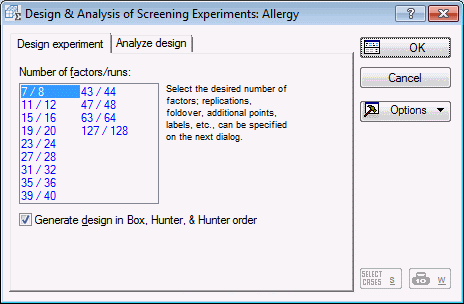
Select the Advanced tab. Select Two-level screening (Plackett-Burman) designs and click OK to display the Design & Analysis of Screening Experiments dialog box.

Saturated 2(k-p) designs. The Design experiment tab lists a selection of highly fractionalized designs. Designs where the number of runs are equal to a power of 2 (e.g., 8, 16, 32, etc.) are saturated factorial designs, where all interactions of a full factorial are aliased with new factors. For example, the 15 factors/16 runs design is actually a 2(15-11) fractional factorial design, that is, it is constructed from a 24 full factorial design, and then all 2-way and 3-way interactions, and the 4-way interaction are used for constructing new factors.

Plackett-Burman designs

Plackett and Burman (1946) showed how full factorial designs can be fractionalized in a different manner, to yield saturated designs where the number of runs is a multiple of 4, rather than a power of 2. These designs are also sometimes call Hadamard matrix designs.

For this study, we want to screen 35 factors, which we can accomplish in 36 runs by choosing the 35/36 Plackett-Burman design. Click on that design now, and then click OK (or double-click on the design) to display the Design of a Screening (Plackett-Burman) Experiment dialog box.

Specifying factor names and settings

The options for reviewing and enhancing the design are the same as to those reviewed in Example 1.1 for 2(k-p) designs.

The first thing to do is to specify the factor names and settings. Click the Change factor names, values, etc. button, and enter the factor names for this experiment (we will accept the default values, that is, the ±1 codes).

All factors will be treated as continuous (leave the default C in the last column); later, we will append 4 center point runs to estimate the error variability for the dependent variable. Now click OK to accept these factor names and settings.

Adding center points

Select the Add to design tab and enter 4 in the Number of center points (per block) box. For center points runs, we will set all factors at some standard center point value. For example, we will set the room temperature (factor Roomtemp) in between the low and high settings, sleep a medium number of hours, eat a medium breakfast, etc.

Reviewing and saving the design

Select the Quick tab, and click the Summary: Display design button.

You should always randomize the runs for the final experiment to minimize the possibility that some systematic changes in the dependent variable over the consecutive runs will bias your estimates.

Select the Display design tab, and ensure that the Random option button in the Order of runs group box is selected. Note that the random number Seed will be different every time you run the program. This number will be used as a so-called seed for the random number generator. If you want to reproduce an exact order of runs that you have previously produced, you need to set the random number Seed to the previous value. However, normally you can simply accept the default seed.

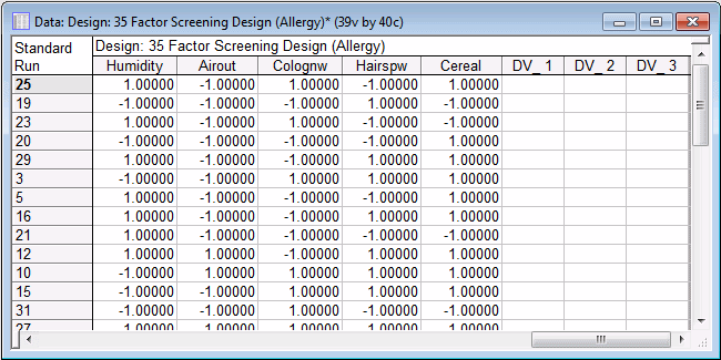
For the final experiment, we want to add 3 blank columns so we can print the spreadsheet and use it as a data entry form (as the dependent variables, we will record subjective ratings of 1) difficulty of breathing, 2) watering of eyes, and 3) feeling of overall fatigue).

Click on the Add to design tab and enter 3 in the Number of blank columns (dep. vars) box.

Now click the Summary: Display design button again.

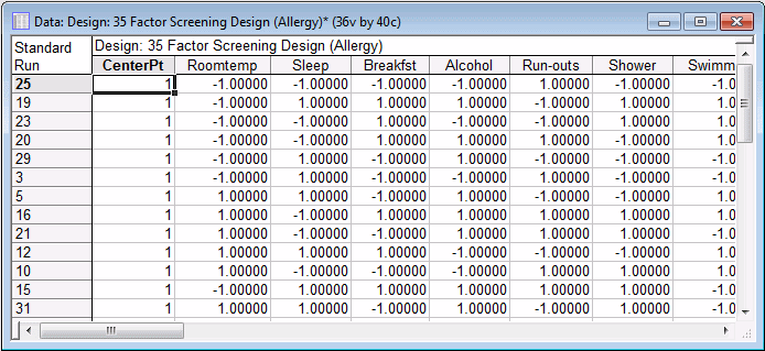
In the spreadsheet above, only the right-most columns are shown. Note that the order of runs is randomized, and the center points appear randomly distributed across the runs. Overall, the design now has 36 (standard runs) + 4 (center points) = 40 runs. Thus, the entire experiment can be completed in 8 weeks (at one run per working-day).

You can now save the design to use as a standard Statistica data file by choosing Save as from the File menu. Note that a completed data file Allergy.sta is already included as an example data file.

Analyzing the experiment

Specifying the design

The example data file Allergy.sta contains the design as well as values for the dependent variables. Those variables were the subjective daily ratings 1) difficulty breathing (variable Breathng), 2) watering eyes (Watereye), and 3) overall fatigue (Fatigue). The ratings were made on a scale from 1 to 100.

To analyze the experiment, open the data file Allergy.sta.

Start the Experimental Design module. In the Design & Analysis of Experiments Startup Panel, select the Advanced tab.

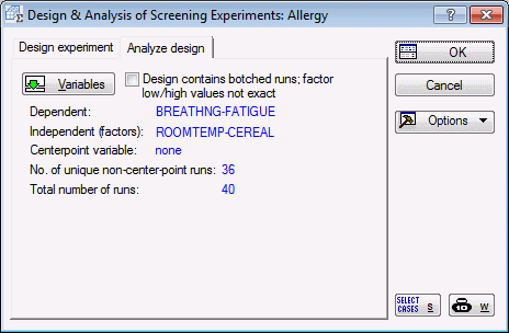
Select Two-level screening (Plackett-Burman) designs and click OK to display the Design & Analysis of Screening Experiments dialog box. Select the Analyze design tab, and click the Variables button. In the variable selection dialog box, select Breathng, Watereye, and Fatigue as the Dependent variables; select variables 1 to 35 as the Independent vars (factors). Click the OK button.

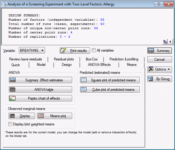
In the Design & Analysis of Screening Experiments dialog box, click OK to display the Analysis of a Screening Experiment with Two-Level Factors dialog box.

Pareto chart of effects

A quick way to screen the 35 factors in this study is to review the Pareto chart of the (standardized) effects. On the Quick tab, click the Pareto chart of effects button in the ANOVA group box.

For the first dependent variable (difficulty breathing), it appears that there are 5 factors that are statistically significant, and clearly have a much larger effect than the other factors: 1) The humidity of the room (the parameter value is negative, thus, the higher the humidity, the less symptoms), 2) whether you jog outside (positive parameter value; running outside increases symptoms), 3) whether you used after-shave (after-shave makes symptoms worse), 4) whether you air out the bedroom in the evening (outside air makes symptoms worse), and 5) whether you pet the cat (petting the cat makes symptoms worse).

Normal probability plot of effects

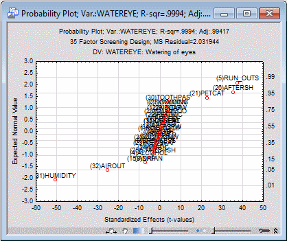
Another plot that helps to quickly sort out the important factors is the normal probability plot of effects. In short, in this plot the effects are ranked, and then plotted against the expected normal probability (or z-value associated with the probability). Small effects that are due to random noise will be distributed with a mean of 0, and a particular standard deviation; those effects will be plotted along a reference line in the graph. Significant "real" effects on the other hand do not "belong" to the distribution of random noise effects with a mean of 0, and will not be plotted along the same line as the random noise effects.

Select the ANOVA/Effects tab. Select the Label points in normal plot check box, select the second dependent variable in the Variable box (Watereye), and click the Normal probability plot button.

Most of the factors are "bunched together" in the center of the plot, along a steep upward sloping line, but the five factors identified as important for the dependent variable are again clearly visible.

Checking the fit of final model

As it turns out, the results for the third dependent variable Fatigue will yield very similar results. Therefore, as the final model, let's fit to the data the simple 5-main-effects model.

In the Analysis of a Screening Experiment with Two-Level Factors dialog box, set the Variable back to the first dependent variable, Breathng.

Select the Model tab. Select the Ignore some effects check box in the Include in model group box. In the Customized (Pooled) dialog box, select to pool all variables together, except for Humidity, Run_outs, Aftersh, Airout, and Petcat. Then click OK.

Select the Curvature check box in the Include in model group box, and select the Pure error option button in the ANOVA error term group box.

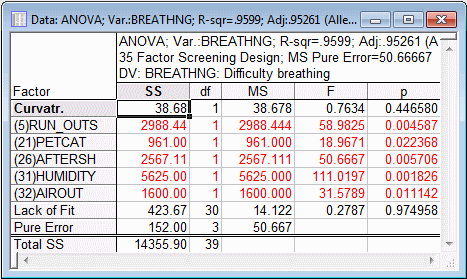
Select the ANOVA/Effects tab and click the ANOVA table button.

The first row of the spreadsheet contains a check for Curvature. This is a test of the difference between the center point runs and the non-center point runs. If significant, then there is reason to believe that the relationship between some of the factors and the dependent variable is not simply linear in nature. The selected main effects are listed in the following rows, and all of them are statistically significant.

Note: these tests are performed against the estimate of Pure Error listed in the next-to-last row. As described in the Introductory Overview, the pure error is estimated from the replicated runs, in this case, the replicated center point runs. It is an estimate of the pure measurement variability (reliability), independent of the variability due to the different factor settings (since it is based on measurements at identical settings of the factors). Therefore, we can test against this estimate of variability the residual variability for all the factors that we pooled together. This is the test of Lack of Fit also shown in the spreadsheet above. In this case, the test does not yield statistical significance, and hence, we can be satisfied that the current model provides a satisfactory fit to the data.

Normal probability plot of residuals

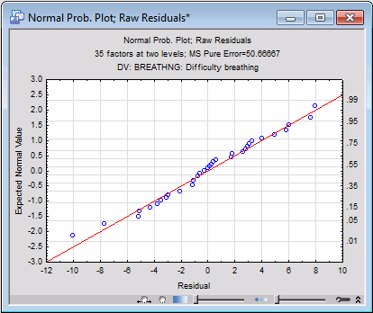
Finally, let's look at the normal probability plot of the residuals for this model by clicking the Normal plot button in the Probability plots of residuals group box on the Residual Plots tab.

The residuals are plotted along a common line, and it appears that they closely follow the normal distribution.

Conclusion

This (fictitious) experiment allowed us to screen a large number of factors for those that were significantly related to the dependent variables of interest. If an industrial process had been studied (instead of the causes of allergies), you could now proceed and further study the important variables as suggested by this experiment.

For example, you could attempt to optimize the process by moving the settings of the important factors further in the direction expected to yield a more desirable outcome. Usually, as you approach the optimum settings for factors, the relationship between the factors and the dependent variable becomes curvilinear (see also Introductory Overview). Thus, you may have to turn to 3-level factorial experiments or central composite design experiments for further experimentation.

See also, Experimental Design Index.