Example 6: Repeated Measures ANOVA Design

This example demonstrates how to set up a repeated measures design with more than one repeated measures factor. How contrast analyses can aid in the interpretation of interaction effects are also shown. The issue of sphericity will be illustrated when the alternative multivariate test of the key interaction is not Statistically significant, while the conventional univariate test indicates significance. The results from the Greenhouse-Geisser and Huynh-Feldt adjustments will be compared to the multivariate test. And finally, the nature and cause of the violation of the sphericity assumption will be explained.

Research Problem

This example is based on a (fictitious) data set reported in Winer (1962, page 324). Suppose you are interested in learning how meaningful versus white (non-meaningful) background noise over time affects people's ability to perform a fine-tuning task.

For example, operators of complex industrial machinery (e.g., nuclear power plants) constantly need to read (and process) various gauges and adjust machines (dials) accordingly. It would be interesting to learn how people's performance on this task is affected by white noise (which sounds like the hiss you hear when tuning your radio in between stations) as compared to meaningful background noise (if you tune the radio to an actual station).

This will be simulated in an experiment in which subjects are required to adjust one of three different dials whenever the respective gauge indicates a significant deviation from specification. Some subjects will perform this task under white background noise conditions, while others will perform it under meaningful background noise (e.g., a radio news program). The dependent measure is the number of errors that the subjects make (failure to set a dial properly within a short tolerance period) during three consecutive 10-minute time intervals.

The resulting design is a 2 (Noise condition) by 3 (Time periods of 10 minutes each) by 3 (Dials; the three dials) analysis of variance. The last two factors are within-subject or repeated measures factors because they represent repeated measurements on the same subject; the first factor is a between-groups factor because subjects will be randomly assigned to work under one or the other noise condition.

The setup of a data file for repeated measures analysis is straightforward: The between-groups factor (Noise condition) can be specified as before, that is, a variable is set up containing the codes that uniquely identify to which experimental condition each subject belongs. Each repeated measurement is then put into a different variable.

It may be convenient to order those variables in a meaningful manner, but no special order is necessary because the GLM module allows you great flexibility in specifying the levels of the repeated measures factors. In this example data file, there are 6 subjects (3 in each group), and the order of variables are arranged so that for each successive time period the measurements for each dial are placed next to each other. The next image shows the data file Dials.sta.

Ribbon bar. Select the Home tab. In the File group, click the Open arrow and select Open Examples to display the Open a Statistica Data File dialog box. Open the data file, which is located in the Datasets folder. Then, select the Statistics tab. In the Advanced/Multivariate group, click Advanced Models and from the menu, select General Linear to display the General Linear Models (GLM) Startup Panel.

Classic menus. From the File menu, select Open Examples to display the Open a Statistica Data File dialog box. Open the data file, which is located in the Datasets folder. Then, from the Statistics - Advanced Linear/Nonlinear Models submenu, select General Linear Models to display the General Linear Models (GLM) Startup Panel.

In the Type of analysis box, select Repeated measures ANOVA. In the Specification method box, select Quick specs dialog. Then, click the OK button to display the GLM Repeated Measures ANOVA Quick Specs dialog box.

Click the Variables button to display a standard variable selection dialog box.

Select variables 2 - 10 (Tim1_Dl1 to Tim3_Dl3) in the Dependent variable list (repeated measures variables). Select variable 1 (Noise) as the Categorical predictor (factors), and then click the OK button.

Next, click the Factor codes button and select the codes (MEANGFLL and WHITE) for the categorical predictor variable by clicking the All button and then the OK button.

Repeated measures factors in the GLM module are always specified in the following manner. First, you specify how many repeated measures factors there are; next, you name those factors and specify their levels. Statistica will later divide the dependent variable list by cycling through the specified levels for each repeated measures factor, and assign successive variables from the dependent variable list to the levels of the repeated measures factors. When cycling through the levels of the repeated measures factors, the fastest changing "subscript" is that of the last specified factor, the next-to-the-last specified factor, and so on; see also Specifying within-subject factors, Specifying more than one repeated measures factor, or Multivariate repeated measures designs for a detailed description of how to specify repeated measures factors.

In this example, there are two repeated measures factors: 1) the three successive 10-minute time periods, and 2) the three dials. To specify these factors, click the Within effects button, and in the resulting Specify within-subjects factors dialog box, specify the repeated measures factor names and their levels, as described below.

When you look at the data file, the slowest changing subscript in the list of variables is that specifying the levels of the Time factor. To clarify the term "subscript," look back at the spreadsheet of the data file, and while moving your finger over the list beginning with variable Tim1_Dl1 say out loud "one two three one two three one two three." Each "one" in this case points to a variable that contains data for the first dial (Dl1), each "two" for the second dial (Dl2), and each "three" for the third dial (Dl3). Thus, the fastest changing subscript is that of factor Dial, and you must specify that factor last. Consequently, factor Time must be specified first.

Thus, in the Specify within-subjects factors dialog box, enter 3 as the No. of levels and TIME as the first Factor Name; likewise, enter 3 as the No. of levels for the second Factor Name - DIALS.

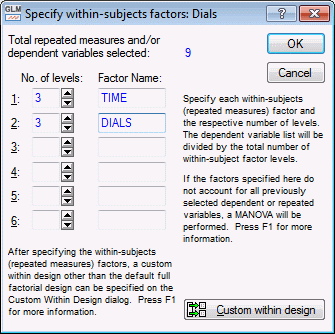
You have now specified the within-subject (repeated measures) part of the design; click the OK button to return to the GLM Repeated Measures ANOVA Quick Specs dialog box.

To view the syntax program automatically generated from the specifications, click the Syntax editor button in the lower-right corner of the GLM Repeated Measures ANOVA Quick Specs dialog box to display the GLM Analysis Syntax Editor.

The remainder of the specifications for this analysis can use the default specifications, so click the OK (Run) button in the GLM Analysis Syntax Editor or the OK button in the GLM Repeated Measures ANOVA Quick Specs dialog box to perform the analysis.

When the GLM Results dialog box is displayed, click the All effects/Graphs button to display the Table of All Effects.

In the ANOVA table, there are three significant effects [with an asterisk (*) by the p-value] in this analysis: the main effect for Time, the Time*Noise interaction, and the main effect for Dials. Now, look at the significant interaction.

First, select (i.e., highlight) the Time*Noise interaction, and then select the Spreadsheet option button in the Display group box.

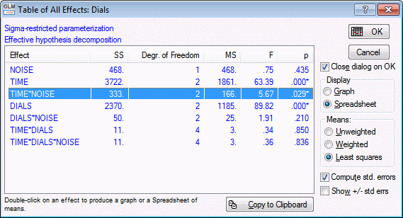
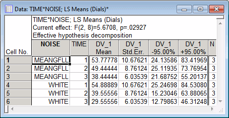
Click the OK button to produce the spreadsheet of marginal means for this effect.

The easiest (and sometimes it seems only) way to understand interactions is to plot them. Therefore, return to the Table of All Effects (click the All effects/Graphs button), and select the Graph option button in the Display group box. Now, click the OK button to display the Arrangement of Factors dialog box.

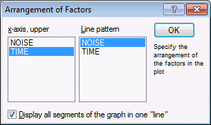
Here you can rearrange the factors for the plot, however, for this example, just click the OK button and accept the default selections.

It appears that in both Noise conditions, subjects' performance improved, that is, they made fewer errors in successive 10-minute trials. However, the two lines denoting the two Noise conditions diverge starting at time period 2 (level_2). It seems that subjects did better (made fewer errors) in the white noise condition than in the meaningful noise condition at Times 2 and 3, but not at Time 1.

You may want to plot the main effect for factor Dials in the same manner. This effect simply shows that for some reason, subjects made more errors adjusting the third dial than the second dial, and more errors adjusting the second dial than the first dial. This effect reflects the differences between the different dials used in the experiment, but it is not of particular theoretical interest in this study. Therefore, now turn to the interaction effect.

We can explore the interaction further by performing a contrast analysis. Return to the GLM Results dialog box, and select the Comps tab to access the options for performing comparisons of means. In general, contrasts are specified in terms of patterns of positive and negative integers that, in a sense, serve as weights. Cells that are assigned integers of different signs are compared (contrasted) in the analysis. See also Planned comparisons of least square means for details.

Note that complex contrasts can also be entered in one long string of contrasts coefficients (instead of separately for each factor, as we will do in this example), by selecting the Together (contrast vectors) option button in the Enter contrasts separately or together group box on the Comps tab.

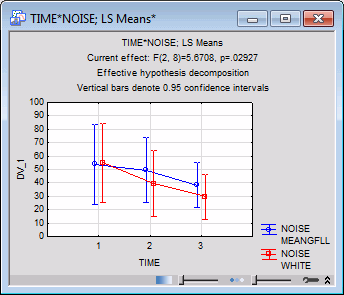
For this example, the difference between the two noise conditions, separately at Times 2 and 3, will be evaluated.

Click the Contrasts for LS means button to display the Specify Contrasts for this Factor dialog box.

First, specify a contrast for factor Noise: enter 1 and -1, respectively (in order to contrast the first level with the second level). Note that instead of typing the values of contrast coefficients, you can use the Quick Fill facility, which enables you to enter the coefficients (into individual cells or entire columns) by clicking the respective buttons.

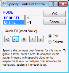
Click the OK button to display the Repeated Measures Factors dialog box, listing each of the repeated measures factors.

In order to enter the contrast for the factor Time, click the Time button. Then enter the coefficients 0, 1, and 0, respectively, in the Enter Contrasts for this Factor dialog box. (Note that you can use the Quick Fill facility, as explained above.)

Click the OK button to return to the Repeated Measures Factors dialog box and similarly click the Dials button. Enter 1, 1, and 1 as the coefficients for this factor. In this manner, you will collapse across all levels of this factor. Because these are the default coefficients, you may also simply click the OK button in the Enter Contrasts for this Factor dialog. Now, click the OK button in the Repeated Measures dialog box to return to the Comps tab. Finally, click the Compute button to produce numerous spreadsheets. In particular, we will look at the Univariate Test of Significance for Planned Comparison spreadsheet.

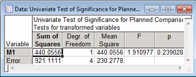
Apparently, the difference between the two means (White vs. Meaningful noise) at Time 2 is not Statistically significant. You may also want to try the comparison between those two groups at Time 3 (for factor Time enter the coefficients 0, 0, 1; all other specifications are the same). That comparison is not significant either.

As it turns out, you cannot say that different types of noise led to significantly different numbers of errors at Time 2 or 3. However, the overall interaction is significant, and, looking back at the plot of the interaction, it looks like the differential changes from Time 1 to Time 2 are mainly responsible for this interaction.

The significance of the interaction between Noise and Time (ignoring the third level of Time, i.e., Time 3) will now be tested. To do this, once again, click the Contrasts for LS means button and specify the contrast coefficients 1 and -1 for the Noise variable in the Specify Contrasts for this Factor dialog box and click the OK button.

Next, enter the coefficients 1, -1, 0, respectively, for factor Time and the coefficients 1, 1, 1 for factor Dials in the Repeated Measures Factors dialog box (see above) and then click the OK button. As you can see, the first two levels of factor Noise and the first two levels of factor Time are being contrasted. Now, click the Compute button to view the spreadsheets.

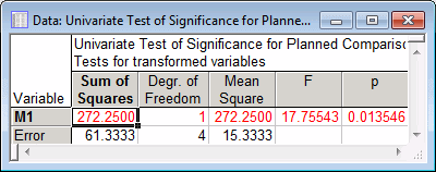
This contrast is Statistically significant. It indeed looks as though the significant two-way interaction between Noise and Time can be traced to the differential changes (improvements) in the number of errors from Time 1 to Time 2 in the White noise condition as compared to the Meaningful condition; subjects in the former condition improved their performance more than subjects in the latter condition.

In some scientific disciplines, the multivariate approach to repeated measures ANOVA with more than two levels has quickly become the only accepted way of analyzing these types of designs. This is because the multivariate approach does not rest on the assumption of sphericity and compound symmetry.

In short, univariate repeated measures ANOVA assumes that the changes across levels are uncorrelated across subjects. This assumption is highly suspect in most cases. In the present example, it is quite conceivable that subjects who improved a lot from Time 1 to Time 2 reached a ceiling in their accuracy, and improved less from Time 2 to Time 3. Given the suspicion that the sphericity assumption for univariate ANOVA has been violated, look at the multivariate statistics.

To produce multivariate tests of significance, select the GLM Results - Summary tab and select all of the check boxes (Pillai's, Hotelling's, and Roy's) in the Multiv. tests group box. Then, click the Multiv. tests button in the Within effects group box. Now, review the multivariate results.

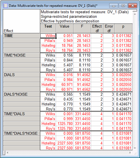
There are different multivariate test criteria; in this case, Wilks' Lambda, Pillai-Bartlett Trace, Hotelling-Lawley Trace, and Roy's Largest Root agree: the interaction is not significant at the .05 level! Thus, here you have a case where the violation of the sphericity assumption led to an erroneous acceptance of the interaction effect as being Statistically significant.

Before the multivariate approach gained popularity, some authors proposed corrections for the univariate F to adjust for violations, notably the Greenhouse-Geisser correction (Greenhouse and Geisser, 1958, 1959) and the Huynh-Feldt correction (Huynh and Feldt, 1976).

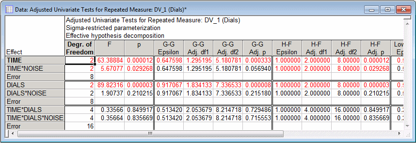
The spreadsheet shows the adjusted univariate tests. As you can see above, the Greenhouse-Geisser adjustment does a "good job" of protecting against erroneously accepting the interaction as Statistically significant at the .05 level. In fact, the p-value for that test (.057) is very similar to that for the multivariate test (p = .062). The Huynh-Feldt adjustment does not help much in this case.

To summarize the analysis of this example, an interaction between Noise and Time emerged between Time 1 and Time 2 (the first and the second 10-minute segment) subjects in the white noise condition improved more (made fewer errors) than subjects in the meaningful noise condition. However, the differences in the number of errors (between groups) are not Statistically significant at any time. Further analyses revealed a serious violation of the sphericity assumption, casting doubt on the initial conclusions. The multivariate test of the interaction between Noise and Time, as well as the Greenhouse-Geisser adjusted univariate test, failed to reach Statistical significance at the .05 level. This example has demonstrated the advantages of using the multivariate approach to repeated measures ANOVA with more than two levels (on the repeated measures).

See also GLM - Index.