Example: Regression Random Forests

The example is based on the data file Poverty.sta. Open this data file via the File - Open Examples menu; it is in the Datasets folder. The data are based on a comparison of 1960 and 1970 Census figures for a random selection of 30 counties. The names of the counties were entered as case names.

The information for each variable is contained in the Variable Specifications Editor (accessible by selecting All Variable Specs from the Data menu).

The purpose of the study is to analyze the correlates of poverty, that is, the variables that best predict the percent of families below the poverty line in a county. Thus, you will treat variable 3 (PT_POOR) as the dependent or criterion variable, and all other variables as the independent or predictor variables.

Select Random Forests for Regression and Classification from the Data Mining menu to display the Random Forest Startup Panel.

Select Regression Analysis as the Type of analysis on the Quick tab, and click OK to display the Random Forest Specifications dialog.

Click the Variables button to display the variable selection dialog.

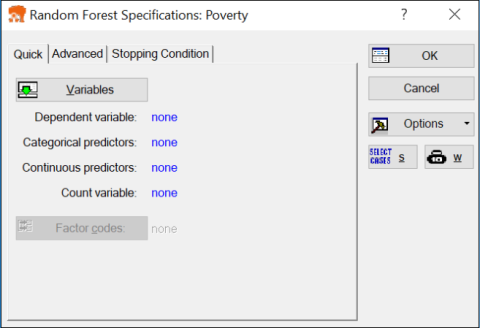
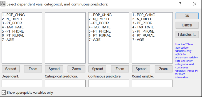
Select PT_POOR as the dependent variable and all others as the continuous predictor variables.

Click the OK button to return to the Random Forest Specifications dialog.

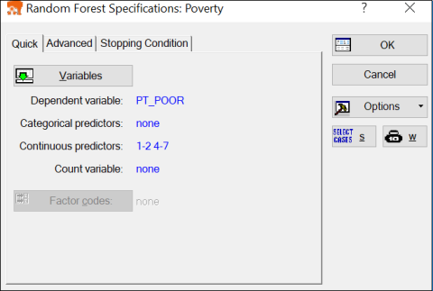
There are a number of additional options available on the Advanced and Stopping condition tabs of this dialog, which can be reconfigured to "fine-tune" the analysis. Click on the Advanced tab to access options to control the number and complexity (number of nodes) of the simple tree models you are about to create.

By default, the Random Forest module partitions the data into training and testing samples by randomly selecting cases from the data set. While the training sample is used to build the model (add simple trees), the testing set is used to validate its performance. This performance is used for validating the model, which for regression tasks is simply defined as the average error. By default, Random Forest selects 30% of the data set as test cases.

Instead of randomly partitioning the data set into training and test cases, you can define your holdout (testing) sample via the Test sample option. When you click the Test sample button, the Test-Sample dialog is displayed where you can identify a sample identifier code that you can use to divide the data into training and testing sets. Selecting this sampling method will override the random sampling option.

One of the advantages of Statistica Random Forest is the ability to perform predictions based on a partial number (subset) of the predictor variables. This feature is particularly attractive for data sets with an extremely large number of predictors.

In particular, you can specify the number of predictor variables you want to include in your tree models. This option is an important one, and care should be taken in setting its value. Including a large number of predictors in the tree models may lead to prolonged computational time and, thus, missing one of the advantages of the Random Forest models, which is the ability to perform predictions based on a subset of the predictor variables. Alternately, including too small a number of predictor variables may downgrade prediction performance since this can exclude variables that may account for most of the variability and trend in the data. In setting the number of predictor variables, it is recommended that you use the default value, based on the formula   (see Breiman for further details).

The options on the Stopping condition tab provide you with an advanced set of criteria for stopping the Random Forest algorithm.

By default, building a Random Forest involves adding a fixed number of trees (default is 100). This is a reasonable approach, especially if you are sitting and watching trees being added to your model, in which case you can always click either the Stop & go to results or Cancel button to abort training if you decide it is not doing well.

However, for longer training runs there may be better ways to specify when training should stop. You can do this on the Stopping Conditions tab. The most useful option is perhaps the Percentage decrease in training error. This states that if the training error does not improve by at least the amount given over a set number of epochs (the Cycles to calculate mean error) then training should stop.

For this example, leave these options at their default settings, and click the OK button on the Random Forest Specifications dialog. The Computing... dialog is displayed, which indicates each step a tree is added to the Random Forest, as well as an estimate of how long the analysis is likely to take.

After all computations are completed, the dialog will automatically close, and the Results dialog will be displayed.

First, click the Summary button to review how consecutive training and testing classification rates progressed over the entire training cycles.

This graph demonstrates the basic mechanism of how the Random Forest algorithm implemented in Statistica can avoid overfitting (see also the Introductory Overview and Technical Notes). In general, as more and more simple trees are added to the model, the misclassification rate for training data (from which the respective trees were estimated) will generally decrease. The same trend should be observed for misclassification rates defined over the testing data. However, as more and more trees are added, the misclassification rate for the testing data will at one point start to increase (while the misclassification rate for the training set keeps decreasing), clearly marking the point where evidence for overfitting is beginning to show.

By default, the program will stop adding trees even if the designated number of trees specified in the Number of trees option on the Advanced tab is not reached. To turn off the stopping condition, simply clear the Enable advanced stopping condition on the Stopping condition tab of the Random Forest Specifications dialog. In this case, the designated number of trees specified in the Number of trees option will added to the Random Forest.

Note that you can generate predictions for any group of data cases of your choice including training, testing, or the entire data set. Also, you can make predictions for partially missing predictor cases, which is one of the capabilities of the Random Forest module (see the Introductory Overview and Technical Notes for further details).

To produce predictions for all the cases in the data set, for example, click on the Prediction tab, select the All samples option button.

Then, in the Sample group box, and click the Predicted values button to display a spreadsheet of the observed, predicted, and residual values.

Other useful graphs to review are Predicted vs. residuals,

Observed vs. predicted,

and Observed vs. residuals. You can generate these graphs by clicking the respective buttons.

In addition, you may want to review the various additional summary statistics (e.g., Risk estimates, available from the Quick tab) and the predictor importance (in the form of a histogram, via the Bargraph of predictor importance button on the Quick tab). The Predictor importance graph contains the importance ranking on a 0-1 scale for each predictor variable in the analysis. See Predictor Importance in Statistica GC&RT, Interactive Trees, and Boosted Trees.

In general, Random Forests (see the Introductory Overview and Technical Notes) is best considered a machine learning algorithm. This module is essentially a "black box," which to some extent will (usually) produce very accurate predictions, but yield models that are not easily interpretable (unlike, for example, classification and regression trees or linear models, where the final prediction model can usually be "put into words," i.e., explained). To interpret the results from the Statistica Random Forest module, there are two key tools:

With the bar graph and spreadsheet of the predictor importance, you can usually distinguish the variables that make the major contributions to the prediction of the dependent variable of interest. Click the Bargraph of predictor importance button on the Quick tab to display a bar graph that pictorially shows the importance ranking on a 0-1 scale for each predictor variable considered in the analysis.

This plot can be used for visual inspection of the relative importance of the predictor variables used in the analysis and, thus, helps to conclude which predictor variable is the most important predictor. See also, Predictor Importance in Statistica GC&RT, Interactive Trees, and Boosted Trees. In this case, variables PT_PHONE, PT_RURAL, and POP_CHNG stand out as the most important predictors.

You can also review the final sequence of trees, either graphically or in a sequence of results spreadsheets (one for each tree). However, this may not be a useful way to examine the "meaning" of the final model when the final solution involves a large number of trees.

Finally, you can deploy the model via the Code generator on the Results dialog - Report tab. In particular, you may want to save the PMML deployment code for the created model, and then use that code via the Rapid Deployment Engine module to predict new cases.

Rather than continually creating new models, which may be time consuming, you can amend your existing Random Forest without full model re-building. Upon analyzing your results, you may find, for example, that your model is not strong enough (i.e., does not fit the data well). In this case, you may want to add more trees by simply specifying the number of trees to add in the Number of more trees option and then clicking the More trees button.