Computing the Optimal Path using Dynamic Time Warping

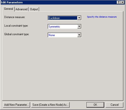
Dynamic Time Warping is a technique for optimally aligning two trajectories. This technique stretches or compresses one or both trajectories in accordance with user specified options such as local and global constraints, so that the trajectories are synchronized.

1. Open a workspace.
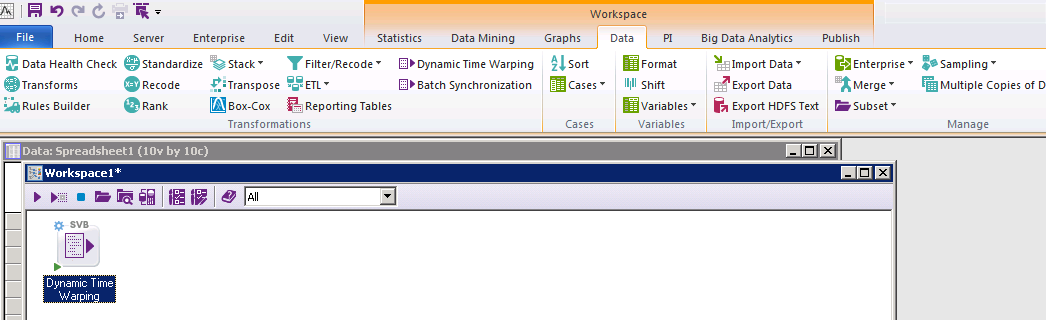
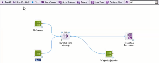
2. On the Data tab, in the Transformations pane, click Dynamic Time Warping.
   This creates a workspace node.

   
3. Select the input spreadsheets which contain the trajectories.
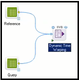
4. To run the algorithm specify the reference and query trajectory.
   

   Note: The specification depends on the ordering of the input nodes. The input spreadsheet that is first connected to the Dynamic Time Warping node is treated as the reference and the input that is connected after connecting the reference node, is treated as the query.
5. Specify the variables for use in the analysis.
   1. Select the Continuous dependent option in the reference spreadsheet to select the variables as inputs to the DTW workspace node.
   2. Select the Continuous dependent option in the query spreadsheet to select the variables as inputs to the DTW workspace node.
6. To open the Edit Parameters dialog box, double-click the Dynamic Time Warping workspace node.
   
7. On the General tab, select the Distance measure along with the local and global constraint types.

   Option	Description
   Distance measure	Select one of the distance measures to be used for computing the distance between the trajectories at each pair of time points. Euclidean distance Squared Euclidean distance Manhattan distance Chebyshev distance Power distance with user defined p and r where p, r can be 1, 2, 3 or 4.
   Local constraint type	Select Symmetric or Asymmetric option from the drop-down list as the local constraint type. Symmetric: Treats both trajectories as equal. There is no distinction between the reference and query trajectories. Both trajectories are mapped to a common time axis. Asymmetric: One trajectory is treated as the reference and the other is the query. In this situation, the query trajectory is mapped to the time axis of the reference trajectory.
   Global constraint type	Select from the following available options: None Sakoe-Chiba: Equidistant band around the main diagonal of the cost matrix with user-defined width. Itakura parallelogram: Parallelogram induced through local transition constraints, which restricts the slope of the path between [1/2, 2].

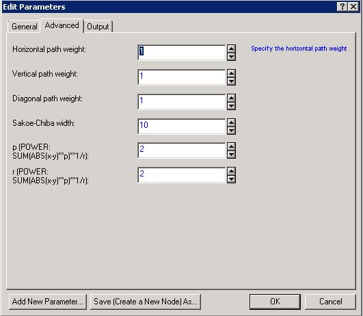
8. On the Advanced tab, specify custom weights for horizontal, vertical, and diagonal moves through the cost matrix.
   

   Note: The Sakoe-Chiba width is available only when you select Sakoe-Chiba as the Global constraint. The power options, p and r, are available only when you select Power as Distance Measure.
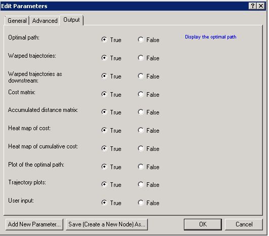
9. On the Output tab, specify the output documents.
   
10. Select True to create a Reporting document for that option.
11. To save the specifications, click OK.

What to do next

Run all nodes in the workspace to get the Warped trajectories and Reporting Documents. Double-click the Reporting Documents to view all the resultant documents and plots.