Building a Regression Model in Spotfire

After you have determined which of the four Spotfire predictive models best suits your data and your desired analysis, use the predictive modeling options available to you from the Tools menu. This example task creates a regression model using sample data.

About this task

From Spotfire, you can build a predictive model that calls TERR for the statistical analysis. In this walkthrough task, build a linear regression model using the Spotfire predictive modeling tools.

For demonstration purposes, use the Baseball Player Statistics data example, available from the Spotfire Library, in Demo/Analysis Files/Baseball. Open the example DXP. (Optionally, use your own suitable data set. )

Before you begin

A Spotfire license for advanced analytics.

Procedure

From the menu, click Tools > Regression Modeling.
Provide a suitable name and descriptive comment for the model.
From the Model method drop-down list, select Linear Regression, and then specify a Data table.
For the example, specify Baseball.
For the Response column, select the response that you want to predict.
For the example, to predict RBI (Runs Batted In), select RBI from the list.
From the Predictor columns box, select all of the variables to consider.
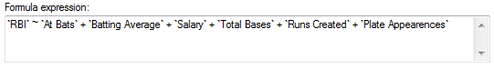
You can select anything that is not a string. Select multiple predictor columns by holding down the control key as you click each one, or click Add for each predictor column you select.

As you click Add, the predictor columns are added to the Formula expression. For the example, the formula expression to model for this example is as follows.
When you have the formula expression for the model, click OK to send the model specification to TERR and create the model.
Spotfire displays the Model page based on your selections.

Review the Model page.


Display	Description
Model Summary	Provides the summary statistics appropriate for the particular model type. These statistics can give an indication of how well the model fits the data. It also displays an icon toolbar (), which you can use to edit the model, to create an evaluation model, to predict from the model, or to duplicate the model to manipulate.
Table of Coefficients	Provides the estimates of the coefficients, a measure of the variability or error of each estimate, and a test statistic ( `t.value` or `z.value` ) of the null hypothesis that the coefficients is zero (in other words, not needed in the model). It also provides a p-value for the statistical test.
Residuals vs. Fitted	Shows the residuals on the Y-axis and the fitted values on the X-axis. Values that have the residual 0 are those that would end up directly on the estimated regression surface. The residuals vs fit plot is commonly used to detect non-linearity, unequal error variances and outliers. When a linear regression model is suitable for a data set, then the residuals are more or less randomly distributed around the 0 line. The formula created in Spotfire creates the following pattern: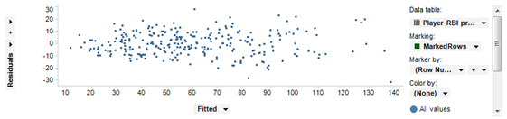
Variable Importance	Shows a summary of the variables that are most relevant for determining the outline. If any of the variables has a very small relevancy, you might want to remove it from the model and rerun the analysis.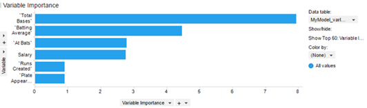

Try duplicating the model and editing the copy to produce different results with different predictor columns.

What to do next

You can create an evaluation model, you can predict from the model, or you can export the model to share with others. See the Spotfire help for more information.