Contents
TIBCO StreamBase provides these high availability services:
-
Synchronous and asynchronous object replication
-
Dynamic object partitioning
-
Application transparent partition failover, restoration, and migration
-
Node quorum support with multi-master detection and avoidance
-
Recovery from multi-master situations with conflict resolution
-
Geographic redundancy
The high availability features are supported using configuration, and are transparent to applications. There are also public APIs available for all of the high availability services to allow more complex high availability requirements to be met by building applications that are aware of the native high availability services. Configuring high availability services is described in the Administration Guide, while programming to the API is described in the Java Developer's Guide.
The remaining sections in the article provide an architectural overview of the high availability services.
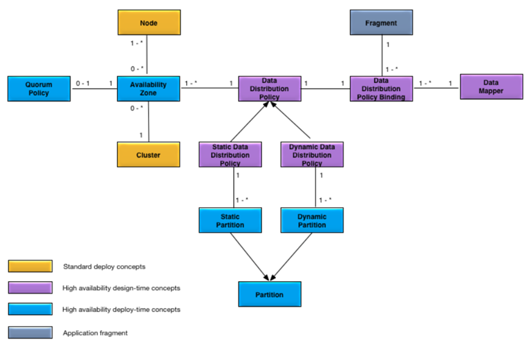
Figure 1, “High availability concepts” shows the high availability concepts added to the standard deployment conceptual model described in Conceptual Model.
-
Availability Zone — a collection of nodes that provide redundancy and quorum for each other.
-
Data Distribution Policy — policy for distributing data across an availability zone.
-
Data Distribution Policy Binding — binds an application data type to a data distribution policy and a data mapper.
-
Data Mapper — implements a specific data distribution policy, such as round-robin, consistent hashing, and so on.
-
Static Data Distribution Policy — a policy that explicitly distributes data across all nodes in an availability zone to ensure optimal data locality. Data is not automatically redistributed as nodes are added and removed.
-
Dynamic Data Distribution Policy — a policy that automatically distributes data evenly across all nodes in an availability zone. Data is automatically redistributed as nodes are added and removed.
-
Partition — the unit of data distribution within a data distribution policy.
-
Static Partition — a partition explicitly defined to distributed data when using a static data distribution policy.
-
Dynamic Partition — a partition created as required to evenly distribute data when using a dynamic data distribution policy.
-
Quorum Policy — a policy, and actions, to prevent a partition from being active on multiple nodes simultaneously.
Each of the concepts in Figure 1, “High availability concepts” is identified as either design time or deploy-time. Design-time concepts are defined in the application definition configuration (see Design Time) and the deploy-time concepts are defined in the node deploy configuration (see Deploy Time).
An availability zone belongs to a single cluster, has one or more nodes, and an optional quorum policy.
A cluster can have zero or more availability zones.
A data distribution policy is associated with one or more availability zones and a data distribution policy binding.
A data distribution policy binding associates a data distribution policy, an application fragment, and a data mapper.
A data mapper is associated with one or more data distribution policy bindings.
An application fragment is associated with one or more data distribution policy bindings.
A dynamic data distribution policy is associated with one or more dynamic partitions.
A dynamic partition is associated with one dynamic data distribution policy.
A node can belong to zero or more availability zones.
A quorum policy is associated with one availability zone.
A partition is associated with one data distribution policy.
A static data distribution policy is associated with one or more static partitions.
A static partition is associated with one static data distribution policy.
A data distribution policy defines how application data is distributed, or partitioned, across multiple nodes. Partitioning of application data allows large application data sets to be distributed across multiple nodes, typically each running on a separate machine. This provides a simple mechanism for applications to grow horizontally by scaling the amount of machine resources available for storing and processing application data. Data distribution policies are associated with one or more availability zones.
To support partitioning application data, an application fragment must be associated with one or more data distribution policies. A data distribution policy defines the following characteristics:
-
How partitions are distributed across available machine resources in an availability zone.
-
The replication requirements for the application data. This includes the replication style, asynchronous versus synchronous, and the number of replica copies of the data.
-
The partitioning algorithm to use to distribute the application data across the available partitions.
Partitions can be distributed across the available machine resources, either dynamically, a dynamic data distribution policy, or statically, a static data distribution policy.
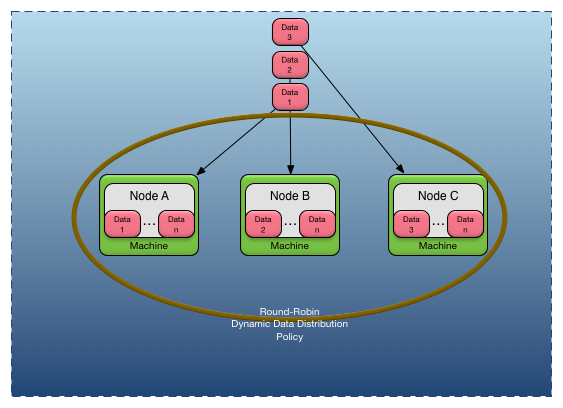
A dynamic data distribution policy automatically creates dynamic partitions based on the available nodes. There is no requirement to explicitly configure dynamic partitions or to map them to specific nodes. Data in a dynamic data distribution policy is automatically redistributed when a node joins or leaves a cluster without any explicit operator action.
Figure 2, “Dynamic data distribution policy” shows a dynamic data distribution policy that provides round-robin data distribution across three nodes. As data is created,
it is assigned to the nodes using a round-robin algorithm: Data 1 is created on Node A, Data 2 is created on Node B, Data 3 is created on Node C, and the next data created is created back on Node A. There are dynamic partitions created to support this data distribution policy, but they are omitted from the diagram since
they are implicitly created by the runtime. If additional nodes are added, the round-robin algorithm includes them when distributing
data.
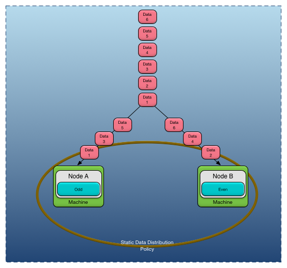
A static data distribution policy requires that static partitions be explicitly configured and mapped to nodes. Data is never repartitioned when using a static data distribution policy. Data can only be migrated to other nodes by loading updated configuration, but the data is never reassigned to a new static partition once it has been created.
Figure 3, “Static data distribution policy” shows a static data distribution policy that uses a data mapper that maps odd data to a partition named Odd and even data to a partition named Even. As data is created it is created on the active node for the partition, so all Odd data is created on Node A and all Even data is created on Node B. Adding a new node to a static distribution policy does not impact where the data is created; it will continue to be created
on the nodes that are hosting the partition to which the data is mapped. Contrast this to the behavior of the dynamic data
distribution policy — where new nodes affect the distribution of the data.
The number of copies of data, or replicas, is defined by a data distribution policy. The policy also defines whether replication should be done synchronously or asynchronously, and other runtime tuning and recovery properties.
Data is distributed across partitions at runtime using a data mapper. A data mapper maps application data to a specific partition at runtime, usually based on the content of the application data. Built-in data mappers are provided, and applications can provide their own data mappers to perform application-specific data mapping.
Figure 4, “Single data center availability zone” shows a simple example of a single cluster with three nodes deployed in a single data center. There is one availability zone defined, which contains all of the nodes in the cluster. The availability zone would define a data distribution policy appropriate for the deployed application, and possibly define a quorum policy that ensures that quorum is always maintained.
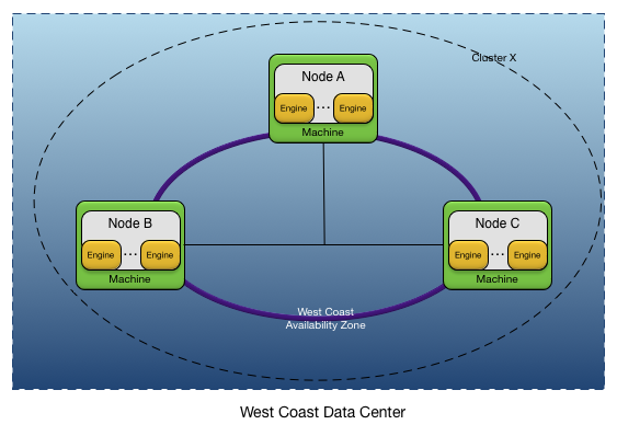
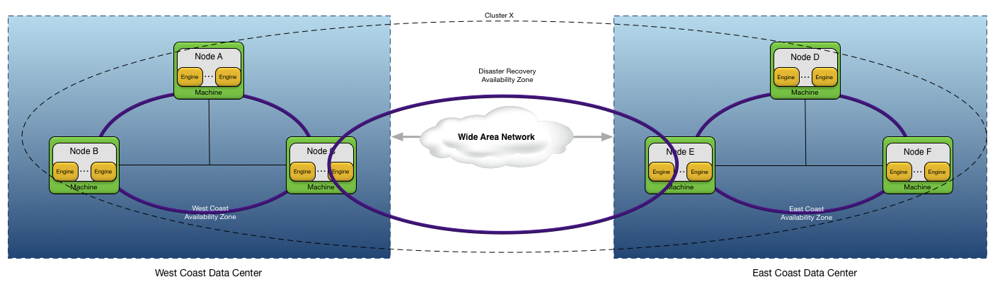
Figure 5, “Disaster recovery (DR) availability zone” shows a more complex example of a cluster that spans two data centers to provide disaster recovery for an application. This examples defines these availability zones:
-
West Coast- availability zone within the west coast data center. -
East Coast- availability zone within the east coast data center. -
Disaster Recovery- availability zone that spans the west and east coast data centers to provide data redundancy across data centers.
Notice that nodes C and E are in multiple availability zones, with each availability zone having possibly different quorum policies.
The application data types that represent the critical application data must be in the same data distribution policy. This
distribution policy is then associated with the Disaster Recovery availability zone to ensure that the data is redundant across data centers.
Partitions provide the unit of data distribution within a data distribution policy.
A partition is identified by a name. Partition names must be globally unique across all nodes in a cluster. Each partition has a node list consisting of one or more nodes. The node list is specified in priority order, with the highest priority available node in the node list the active node for the partition. All other nodes in the node list are replica nodes for the partition. Replica nodes can use either synchronous or asynchronous replication (see Replication).
If the active node becomes unavailable, the next highest available replica node in the node list automatically becomes the active node for the partition.
All data in a partition with replica nodes has a copy of the data transparently maintained on all replica nodes. This data is called replica data.
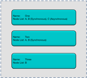
Figure 6, “Partition definitions” defines three partitions named One, Two, and Three. Partitions One and Two support replication of all contained data, with node B replication done synchronously and node C replication done asynchronously. Partition Three has only a single node B defined so there is no replication in this partition. All data assigned to partition Three during creation is transparently created on node BA failure will cause the active node for partition One and Two to change to node BBOne and Two, but it causes all data in partition Three to be lost since there is no other node hosting this partition.
Data is partitioned by installing a data mapper on a managed object using configuration. A managed object with a data mapper installed is called a partitioned object. A data mapper is responsible for assigning a managed object to a partition. Partition assignment occurs:
-
When an object is created.
-
During partition mapping updates (see Updating Object Partition Mapping).
Data mappers are inherited by all subtypes of a parent type. A child type can install a new data mapper to override a parent's data mapper.
A partitioned object is always associated with a single partition, but the partition it is associated with can change during the lifetime of the object.
The algorithm used by a data mapper to assign an object to a partition is application-specific. It can use any of the following criteria to make a partition assignment:
-
Object instance information.
-
System resource utilization (such as CPU, shared memory utilization, and so on).
-
Load balancing (such as consistent hashing, round-robin, priorities, and so on).
-
Any other application-specific criteria.
Built-in data mappers for consistent hashing and round-robin are provided.
The distributed consistent hashing data mapper distributes partitioned objects evenly across all nodes in a cluster, maintaining an even object distribution even as nodes are added or removed from a cluster. When a new node joins a cluster, it takes its share of the objects from the other nodes in the cluster. When a node leaves a cluster, the remaining nodes share the objects that were on the removed node.
Assigning an object to a partition using distributed consistent hashing consists of the following steps:
-
Generate a hash key from data in the object.
-
Access the hash ring buffer location associated with the generated hash key value.
-
Map the object to the partition name stored at the accessed hash ring buffer location.
The important thing about the consistent hashing algorithm is that the same data values consistently map to the same partition.
The size of the hash ring buffer controls the resolution of the object mapping into partitions — a smaller hash ring may cause a lumpy distribution, while a larger hash ring more evenly spreads the objects across all available partitions.
The number of partitions determines the granularity of the data distribution across the nodes in a cluster. The number of partitions also constrains the total number of nodes over which the data can be distributed. For example, if there are only four partitions available, the data can only be distributed across four nodes, no matter how many nodes are in the cluster.
For optimal data distribution, TIBCO recommends sizing the hash ring buffer significantly larger than the number of partitions.
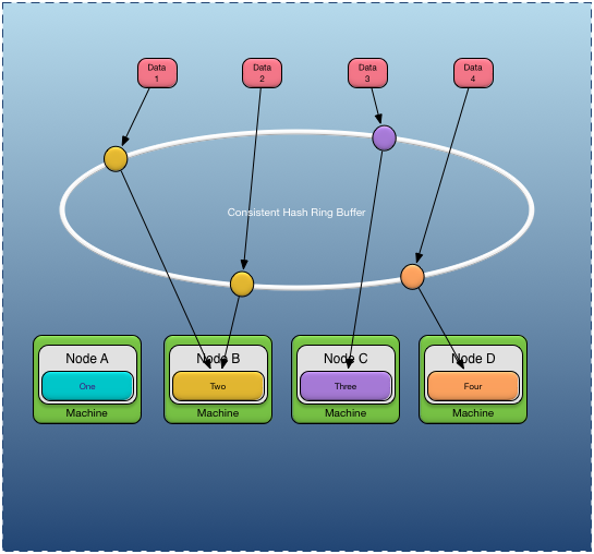
Figure 7, “Distributed consistent hashing” shows an example of mapping data to partitions using distributed consistent hashing. The colored circles on the consistent
hash ring buffer in the diagram represent the hash ring buffer location for a specific hash key value. These locations contain
a partition name. In this example, both Data 1 and Data 2 map to partition Two on node B, while Data 3 maps to partition Three on node C, and Data 4 maps to partition Four on node D.
While the example shows each node only hosting a single partition, this is not realistic, since adding more nodes would not provide better data distribution since there are no additional partitions to migrate to a new node. Real configurations have many partitions assigned to each node.
The round-robin data mapper distributes data evenly across all static partitions, not nodes, in a static data distribution policy. Data is sent in order to each of the partitions defined in the static partition policy.
The distribution of the static partitions across nodes is defined by the partition to node mapping defined by the static data
distribution policy. For example, in Figure 8, “Round-robin data mapper”, two thirds of the data ends up on Node A, since there are two partitions defined on Node A, and only one third on Node B, since Node B has only a single partition defined.
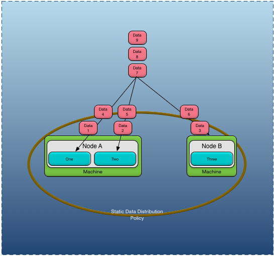
Figure 9, “Foreign partition” shows three nodes, A, B, and C, and a partition P. Partition P is defined with an active node of A and a replica node of B. Partition P is also defined on node C but node C is not in the node list for the partition. On node C, partition P is considered a foreign partition.
The partition state and node list of foreign partitions is maintained as the partition definition changes in the cluster. However, no objects are replicated to these nodes, and these nodes cannot become the active node for the partition. When an object in a foreign partition is created or updated, the create and update is pushed to the active and any replica nodes in the partition.
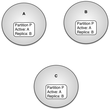
Foreign partition definitions are useful for application-specific mechanisms that require a node to have a distributed view of partition state, without being the active node or participating in replication.
Partitions are defined directly by the application or an administrator on a running system. At minimum, TIBCO recommends defining and enabling partitions (see Enabling and Disabling Partitions) on all nodes on which the partition should be known. This allows an application to:
-
Immediately use a partition. Partitions can be safely used after they are enabled. There is no requirement that the active node has already enabled a partition to use it safely on a replica node.
-
Restore a node following a failure. See Restore for details.
As an example, here are the steps to define a partition P in a cluster with an active node of A and a replica node of B.
-
Nodes A and B are started and have discovered each other.
-
Node A defines partition P with a node list of A, B.
-
Node A enables partition P.
-
Node B defines partition P with a node list of A, B.
-
Node B enables partition P.
You can also redefine partition definitions to allow partition migration to different nodes. See Migrating a Partition for details.
The only time that node list inconsistencies are detected is when object re-partitioning is done (see Updating Object Partition Mapping), or a foreign partition is being defined.
Once a partition is defined, it must be enabled. Enabling a partition causes the local node to transition the partition from
the Initial state to the Active state. Partition activation can include migration of object data from other nodes to the local node. It can also include
updating the active node for the partition in the cluster. Enabling an already Active partition has no effect.
Disabling a partition causes the local node to stop hosting the partition. The local node is removed from the node list in the partition definition on all nodes in the cluster. If the local node is the active node for a partition, the partition migrates to the next node in the node list and becomes active on that node. As part of migrating, all objects in the partition on the local node are removed from shared memory.
When a partition is disabled with only the local node in the node list, there is no impact to the objects contained in the partition on the local node since a partition migration does not occur. The application can continue reading these objects. However, unless the partition mapper is removed, no new objects can be created in the disabled partition because there is no active node for the partition.
When a partition is defined, the partition definition is broadcast to all discovered nodes in the cluster. The RemoteDefined status (see Partition Status) is used to indicate a partition that was remotely defined. When the partition is enabled, the partition status change is again broadcast to all discovered nodes in the cluster. The
RemoteEnabled status (see Partition Status) is used to indicate a partition that was remotely enabled.
While the broadcast of partition definitions and status changes can eliminate the requirement to define and enable partitions on all nodes in a cluster that must be aware of a partition, TIBCO recommends against relying on this behavior in production system deployments.
The example below demonstrates why relying on partition broadcast can cause problems.
-
Nodes
A,B, andCare all started and discover each other. -
Node
Adefines partitionPwith a node list ofA,B,C. Replica nodesBandCrely on the partition broadcast to remotely enable the partition. -
Node
Bis taken out of service. Failover (see Failover) changes the partition node list toA,C. -
Node
Brestarts and all nodes discover each other, but since nodeBdoes not define and enable partitionPduring application initialization, the node list remainsA,C.
At this point, you must intervene manually to redefine partition P to add B back as a replica. This manual intervention is eliminated if all nodes always define and enable all partitions during application
initialization.
A partition with one or more replica nodes defined in its node list fails over if its current active node fails. The next highest priority available node in the node list takes over processing for this partition.
When a node fails, it is removed from the node list for the partition definition in the cluster. All undiscovered nodes in
the node list for the partition are also removed from the partition definition. For example, if node A fails with the partition definitions in Figure 6, “Partition definitions” active, the node list is updated to remove node A leaving these partition definitions active in the cluster.
Once a node is removed from the node list for a partition, no communication occurs to that node for the partition.
A node is restored to service by defining and enabling all partitions that will be hosted on the node. This includes partitions for which the node being restored is the active or replica node. When a partition is enabled on the node being restored partition migration occurs, which copies all objects in the hosted partitions to the node.
Restoring node A to service after the failure in Failover requires the following steps:
-
Define and enable partition
Onewith active nodeAand replicasBandC. -
Define and enable partition
Twowith active nodeAand replicaB.
After these steps execute and partition migration completes, node A is back online and the partition definitions are back to the original definitions in Figure 6, “Partition definitions”.
Partitions have one of the following states:
Partition states
Figure 11, “Partition state machine” shows the state machine that controls the transitions between all of these states.
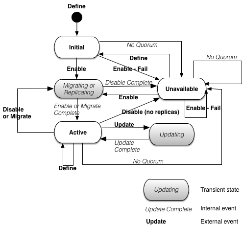
The external events in the state machine map to an API call or an epadmin command. The internal events are generated as part of node processing.
Partition state change notifiers are called at partition state transitions if an application installs them. Partition state change notifiers are called in these cases:
-
The transition into and out of the transient states defined in Figure 11, “Partition state machine”. These notifiers are called on every node in the cluster that has the notifiers installed and the partition defined and enabled.
-
The transition directly from the
Activestate to theUnavailablestate in Figure 11, “Partition state machine”. These notifiers are only called on the local node on which this state transition occurred.
Partitions also have a status, which defines how the local definition of the partition was done, and whether it was enabled. The valid states are defined in Partition status.
Partition status
Partition status values are controlled by an administrative operation, or API, on the local node except for the RemoteEnabled and RemoteDefined statuses. The RemoteEnabled and RemoteDefined statuses occurs when local partition state was not defined and enabled on the local node; it was only updated on a remote
node.
If the local node leaves the cluster and is restarted, it must redefine and enable a partition locally before rejoining the cluster to rejoin as a member of the partition. For this reason TIBCO recommends that all nodes perform define and enable for all partitions in which they participate, even if they are a replica node in the partition.
Partitioned objects are replicated to multiple nodes based on the node list in their partition definition. Objects that are replicated to one or more nodes are highly available and are available to the application following a node failure.
Replication can be synchronous or asynchronous on a per-node basis in a partition. A mix of synchronous and asynchronous replication
within the same partition is also supported. For example, in Figure 6, “Partition definitions”, partition One is defined to use synchronous replication to node B and asynchronous replication to node C.
Synchronous replication guarantees that all replica nodes are updated in the same transaction in which the replicated object was modified. There can be no loss of data. However, the latency to update all of the replica nodes is part of the initiating transaction. By default, synchronous replication uses the deferred write protocol described in Deferred Write Protocol.
Asynchronous replication guarantees that any modified objects are queued in a separate transaction. The object queue is per node and is maintained on the same node on which the modification occurred. Modified objects are updated on the replica nodes in the same order in which the modification occurred in the original transaction. The advantage of asynchronous replication is that it removes the update latency from the initiating transaction. However, there is potential for data loss if a failure occurs on the initiating node before the queued modifications have been replicated.
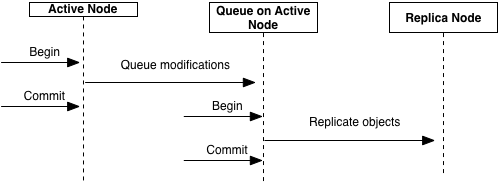
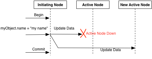
Figure 12, “Asynchronous replication” shows asynchronous replication behavior when a modification is made on the active node for a partition. The following steps are taken in this diagram:
-
A transaction is started.
-
Replicated objects are modified on the active node.
-
The modified objects are transactionally queued on the active node.
-
The transaction commits.
-
A separate transaction is started on the active node to replicate the objects to the target replica node.
-
The transaction is committed after all queued object modifications are replicated to the target node.
Because asynchronous replication is done in a separate transaction consistency errors can occur. When consistency errors are detected they are ignored, the replicated object is discarded, and a warning message is generated. These errors include:
-
Duplicate keys.
-
Duplicate object references caused by creates on an asynchronous replica.
-
Invalid object references caused by deletes on an asynchronous replica.
All other object modifications in the transaction are performed when consistency errors are detected.
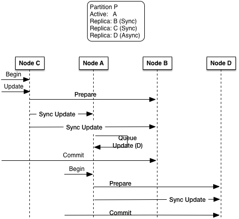
Figure 13, “Replication protocol” provides more details on the differences between synchronous and asynchronous replication. The key things to notice are:
-
Synchronous modifications (creates, deletes, and updates) are always used when updating the active node and any synchronous replica nodes.
-
Modifications to asynchronous replica nodes are always done from the active node, this is true even for modifications done on asynchronous replica nodes.
TIBCO strongly recommends that you do not modify asynchronous replica nodes since there are no transactional integrity guarantees between when the modification occurs on the asynchronous replica and when it is reapplied from the active node.
-
Synchronous updates are always done from the node on which the modification occurred — this can be the active or a replica node.
These cases are shown in Figure 13, “Replication protocol”. These steps are shown in the diagram for a partition P with the specified node list:
-
A transaction is started on node
C— a replica node. -
A replicated object in partition P is modified on node
C. -
When the transaction is committed on node
C, the update is synchronously done on nodeA(the active node) and nodeB(a synchronous replica). -
Node
A(the active node) queues the update for nodeD- an asynchronous replica node. -
A new transaction is started on node
Aand the update is applied to nodeD.
If an I/O error is detected when attempting to send creates, updates, or deletes to a replica node, an error is logged on the node initiating the replication and the object modifications for the replica node are discarded. The replica node is removed from the node list for the partition. These errors include:
-
The replica node has not been discovered yet
-
The replica node is down
-
An error occurred while sending the modifications
The replica node is then re-synchronized with the active node when the replica node is restored (see Restore).
Partitioned objects can be re-partitioned on an active system. This provides a mechanism for mapping objects to new partitions.
The partition mapping for objects is updated using an administrative command or an API. Partition mapping updates can only be initiated on the active node for a partition. When the partition update is requested an audit is performed to ensure that the node list is consistent for all discovered nodes in the cluster. This audit is done to ensure that no object data is migrated to other nodes as part of remapping the partitions.
When a partition update is requested, all installed partition mappers on the active node are called for all partitioned objects. The objects will be moved to the partition returned by the partition mapper.
Warning
Object partition mapping updates only occur if the partition mapper installed by the application supports a dynamic mapping of objects to partitions. If the partition mapper only supports a static mapping of objects to partitions no remapping will occur.
You can install new partition mappers on a node to perform partition updates as shown in these steps:
-
Define and enable a new partition on the local node.
-
Install a new partition mapper that maps objects to the new partition.
-
Perform the partition update.
-
Optionally migrate the partition as needed.
This technique has the advantage that objects created while the partition update is executing are mapped to the new partition.
Partitions support migration to different nodes without requiring system downtime. Partition migration is initiated using an epadmin command or an API on the current active node for the partition. Make the following changes to a partition definition as needed:
-
Change the priority of the node list, including the active node.
-
Add new nodes to the node list.
-
Remove nodes from the node list.
-
Update partition properties.
When you initiate the partition migration all object data is copied as required to support the updated partition definition. This may include changing the active node for the partition.
For example, these steps migrate the active node from A to C for partition P:
-
Node
Cdefines partitionPwith a node list ofC,B. -
Node
Cenables the partition and partitionPmigrates to nodeC.
When the partition migration completes, partition P is now active on node C with node B still the replica. Node A is no longer hosting this partition.
It is also possible to force replication to all replica nodes during a partition migration by setting the force replication property when initiating partition migration. Setting the force replication property causes all replica nodes to resynchronize with the active node during partition migration. In general, forcing replication is not required since replica nodes resynchronize with the active node when partitions are defined and enabled on the replica node.
As discussed in Location Transparency, partitioned objects are also distributed objects. This provides application-transparent access to the current active node for a partition. Applications simply create objects, read and modify object fields, and invoke methods. The StreamBase Runtime ensures that the action occurs on the current active node for the partition associated with the object.
If an active node fails, and the partition is migrated to a new active node, the failover to the new active node is transparent to the application. No creates, updates, or method invocations are lost during partition failover as long as the node that initiated the transaction was not the failing node. Failover processing is performed in a single transaction to ensure that it is atomic. See Figure 14, “Partition failover handling”.
When a partition is migrated to a new active node, all objects in the partition must be write-locked on both the new and old active nodes, and all replica nodes. This ensures that the objects are not modified as they migrate to the new node.
When an object is copied to a new node, either because the active node is changing, or a replica node changed, a write lock is taken on the current active node and a write lock is taken on the replica node. This ensures that the object is not modified during the copy operation.
To minimize the amount of locking during an object migration, separate transactions are used to perform the remote copy operations. The objects locked per transaction partition property sets the number of objects copied in a single transaction. Minimizing the number of objects locked in a single transaction during object migration minimizes application lock contention with the object locking required by object migration.
StreamBase uses a quorum mechanism to detect, and optionally, prevent partitions from becoming active on multiple nodes. Quorums are defined per availability zone. When a partition is active on multiple nodes a multiple master, or split-brain, scenario has occurred. A partition can become active on multiple nodes when connectivity between one or more nodes in a cluster is lost, but the nodes themselves remain active. Connectivity between nodes can be lost for a variety of reasons, including network router, network interface card, or cable failures.
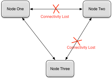
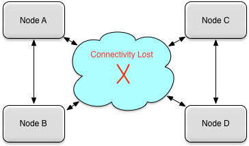
Figure 15, “Multi-master scenario” shows a situation where a partition may be active on multiple nodes if partitions exist that have all of these nodes in their
node list. In this case, Node Two assumes that Node One and Node Three are down, and makes itself the active node for these partitions. A similar thing happens on Node One and Node Three — they assume Node Two is down and take over any partitions that were active on Node Two. At this point these partitions have multiple active nodes that are unaware of each other.
The node quorum mechanism provides these mutually exclusive methods to determine whether a node quorum exists:
When using voting percentages, the node quorum is not met when the percentage of votes in a cluster drops below the configured node quorum percentage. When using minimum number of votes, the node quorum is not met when the total number of votes in a cluster drops below the configured minimum vote count. By default each node is assigned one vote. However, this can be changed using configuration. This allows certain nodes to be given more weight in the node quorum calculation by assigning them a larger number of votes.
When node quorum monitoring is enabled, high availability services are Disabled and the node is taken offline if a node quorum is not met for any availability zones in which a node is participating. This
is true even if the node still has quorum in other availability zones. This ensures that partitions can never be active on
multiple nodes. When a node quorum is restored, by remote nodes being rediscovered, the node state is set to Partial or Active depending on the number of active remote nodes and the node quorum mechanism being used. See Node Quorum States for complete details on node quorum states.
See the StreamBase Administration Guide for details on designing and configuring node quorum support.
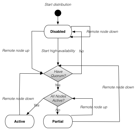
The valid node quorum states are defined in Node quorum states.
Node quorum states
Figure 16, “Quorum state machine” shows the state machine that controls the transitions between all of the node quorum states.
There are cases where disabling node quorum is desired. Examples are:
-
Network connectivity and external routing ensures that requests are always targeted at the same node if it is available.
-
Geographic redundancy, where the loss of a WAN should not bring down the local nodes.
To support these cases, the node quorum mechanism can be disabled using configuration (see the StreamBase Administration Guide). When node quorum is disabled, high availability services are never disabled on a node because of a lack of quorum. With
the node quorum mechanism disabled, a node can only be in the Active or Partial node quorum states defined in Node quorum states — it never transitions to the Disabled state. Because of this, it is possible that partitions may have multiple active nodes simultaneously.
This section describes how to restore a cluster following a multi-master scenario. These terms are used to describe the roles nodes play in restoring after a multi-master scenario:
-
source — the source of the object data. The object data from the initiating node is merged on this node. Installed compensation triggers are executed on this node.
-
initiating — the node that initiated the restore operation. The object data on this node is replaced with the data from the source node.
To recover partitions that were active on multiple nodes, support is provided for merging objects using an application implemented compensation trigger. If a conflict is detected, the compensation trigger is executed on the source node to allow conflict resolution.
The detectable conflicts types are:
-
Instance Added — an instance exists on the initiating node, but not on the source node.
-
Key Conflict — the same key value exists on both the initiating and source nodes, but they are different instances.
-
State Conflict — the same instance exists on both the initiating and source nodes, but the data is different.
The application-implemented compensation trigger is always executed on the source node. The compensation trigger has access to data from the initiating and source nodes.
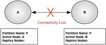
Figure 17, “Active cluster” shows an example cluster with a single partition, P, that has node A as the active node and node B as the replica node.
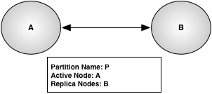
Figure 18, “Failed cluster” shows the same cluster after connectivity is lost between node A and node B with node quorum disabled. The partition P definition on node A has been updated to remove node B as a replica because it is no longer possible to communicate with node B. Node B removes node A from the partition definition because it believes that node A failed, so it has taken over responsibility for partition P.
Once connectivity was restored between all nodes in the cluster, and the nodes have discovered each other, the operator can
initiate the restore of the cluster. The restore (see Restore) is initiated on the initiating node which is node A in this example. All partitions on the initiating node are merged with the same partitions on the source nodes on which the partitions are also active. In the case where a partition was active on multiple remote nodes, the node
to merge from can be specified per partition, when the restore is initiated. If no remote node is specified for a partition,
the last remote node to respond to the Is partition(n) active? request (see Figure 19, “Merge operation - using broadcast partition discovery”) will be the source node.
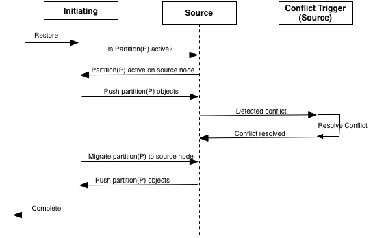
Figure 19, “Merge operation - using broadcast partition discovery” shows the steps taken to restore the nodes in Figure 18, “Failed cluster”. The restore command is executed on node A which is acting as the initiating node. Node B is acting as the source node in this example.
The steps in Figure 19, “Merge operation - using broadcast partition discovery” are:
-
Operator requests restore on
A. -
Asends a broadcast to the cluster to determine which other nodes have partitionPactive. -
Bresponds that partitionPis active on it. -
Asends all objects in partitionPtoB. -
Bcompares all of the objects received fromAwith its local objects in partitionP. If there is a conflict, any application reconciliation triggers are executed. See Default Conflict Resolution for default conflict resolution behavior if no application reconciliation triggers are installed. -
AnotifiesBthat it is taking over partitionP. This is done since nodeAshould be the active node after the restore is complete. -
Bpushes all objects in partitionPtoAand sets the new active node for partitionPtoA. -
The restore command completes with
Aas the new active node for partitionP(Figure 17, “Active cluster”).
The steps to restore a node, when the restore from node was specified in the restore operation are very similar to the ones above, except that instead of a broadcast to find the source node, a request is sent directly to the specified source node.
The example in this section has the A node as the final active node for the partition. However, there is no requirement that this is the case. The active node for a partition could be any other node in the cluster after the restore completes, including the source node.
Figure 20, “Split cluster” shows another possible multi-master scenario where the network outage causes a cluster to be split into multiple sub-clusters. In this diagram there are two sub-clusters:
-
Sub-cluster one contains nodes A and B
-
Sub-cluster two contains nodes C and C
To restore this cluster, the operator must decide which sub-cluster nodes should be treated as the initiating nodes and restore from the source nodes in the other sub-cluster. The steps to restore the individual nodes are identical to the ones described above.
Note
StreamBase does not require that the initiating and source nodes span sub-cluster boundaries. The source and initiating nodes can be in the same sub-clusters.
The default conflict resolution behavior if no compensation triggers are installed is:
You can use the StreamBase high availability features across a WAN to support application deployment topologies that require geographic redundancy, without any additional hardware or software. The same transactional guarantees are provided to nodes communicating over a WAN, as are provided over a LAN.
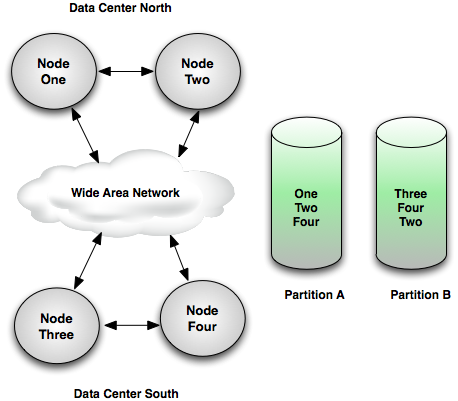
Figure 21, “Geographic redundancy” shows an example system configuration that replicates partitions across the WAN so that separate data centers can take over should one completely fail. This example system configuration defines:
-
Partition
Awith node listOne,Two,Four -
Partition
Bwith node listThree,Four,Two
Under normal operation partition A's active node is One, highly available objects are replicated to node Two, and across the WAN to node Four; partition B's active node is Three, and highly available objects are replicated to node Four and across the WAN to node Two. In the case of a Data Center North outage, partition A will transition to being active on node Four in Data Center South. In the case of a Data Center South outage, partition B will transition to being active on node Two in Data Center North.
Consider the following when deploying geographically redundant application nodes:
-
Network latency between locations. This network latency affects the transaction latency for every partitioned object modification in partitions that span the WAN.
-
Total network bandwidth between locations. The network bandwidth must be able to sustain the total throughput of all of the simultaneous transactions at each location that require replication across the WAN.
Configure geographically distributed nodes to use the static discovery protocol described in Location Discovery.