Example: Goodness of Fit Indices for Regression Predictions
This example is based on Example 1: Standard Regression Analysis from the Multiple Regression module. The example uses the data file Poverty.sta, which contains data pertaining to the comparison of 1960 and 1970 Census figures for a random selection of 30 counties. The names of the counties were entered as case names.
- Research question
- The purpose of the study was to analyze the correlates of poverty, that is, the variables that best predict the percent of families below the poverty line in a county. Thus, in the regression analysis, variable 3 (Pt_Poor) was treated as the dependent or criterion variable, and all other variables as the independent or predictor variables.
- Regression analysis
- Follow Example 1: Standard Regression Analysis in the Multiple Regression module to the point where the spreadsheet with predicted and residual values is computed. Then, on the Save tab of the Residual Analysis dialog box, click the Save residuals & predicted button.
After selecting that option, make sure to select variable 3 Pt_Poor as an additional variable to save in the Select variables to save with predicted/residuals scores dialog box.
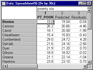
The resulting spreadsheet should then contain the observed and predicted values computed from the regression analysis (along with various other residual statistics).
- Goodness of fit computations
- Next select Goodness of Fit, Classification, Prediction from the Data Mining menu to display the
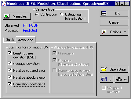
Goodness of Fit, Classification, Prediction Startup Panel. Ensure that the newly created spreadsheet with the observed and predicted values from the regression analysis is indeed the one selected for the analysis; if it is not, use option Open Data to select that spreadsheet. Click the Variables button and select variable Pt_Poor as the variable with observed values, and variable Predicted as the variable with predicted values. Next, on the
Advanced tab of the Startup Panel, select all Statistics for continuous DV.
Next, click OK to display the Results dialog box, and click the Summary goodness of fit measures button.
Note: the Correlation coefficient computed for the observed and predicted values is identical to the multiple correlation computed by the analysis discussed in Example 1 of Multiple Regression. However, because the Goodness of Fit module does not "know" that the predicted values were computed via multiple regression, the Mean square error is the actual mean of the sums of squared deviations of the predicted from the observed values. For comparison, you may want to display the ANOVA table in the Multiple Regression module; you will see that the mean square error reported there is slightly different, because that value is computed as the sum of squares deviation divided by the degrees of freedom for the residuals (from the regression analysis).The main utility of the Goodness of Fit module is that it allows you to quickly compute various indices of goodness of fit (as further described in Computational Details), for different models and for different analyses. For example, we could now use other statistical techniques (e.g., see Example 2: Regression Tree for Predicting Poverty of the General Classification and Regression Trees module) to compute predicted values, and compute the same fit indices, to compare the goodness of fit of the prediction from different models. For an example (for a classification problem) of how these computations can be useful when evaluating (competing) models for predictive classification in a data mining project, see Example 4: Predictive Data Mining for Categorical Output Variable (Classification) in the STATISTICA Data Miner examples section.


