Example 2: Prediction of Continuous Dependent Variable
This example is based on a re-analysis of the data presented in Example 1: Standard Regression Analysis for the Multiple Regression module, as well as Example 2: Regression Tree for Predicting Poverty for the General Classification and Regression Trees module.
The example is based on the data file Poverty.sta. Open this data file via the File - Open Examples menu; it is in the Datasets folder. The data are based on a comparison of 1960 and 1970 Census figures for a random selection of 30 counties. The names of the counties were entered as case names.
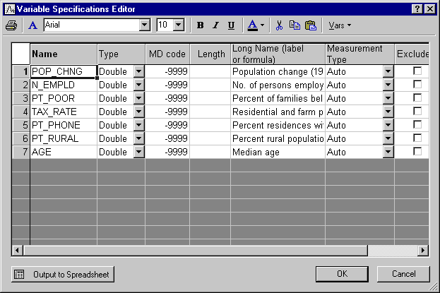
The following information for each variable is contained in the Variable Specifications Editor (accessible by selecting All Variable Specs from the Data menu).
- Research Question
- The purpose of the study is to analyze the correlates of poverty, that is, the variables that best predict the percent of families below the poverty line in a county. Thus, you will treat variable 3 (Pt_Poor) as the dependent or criterion variable, and all other variables as the independent or predictor variables.
- Setting Up the Analysis
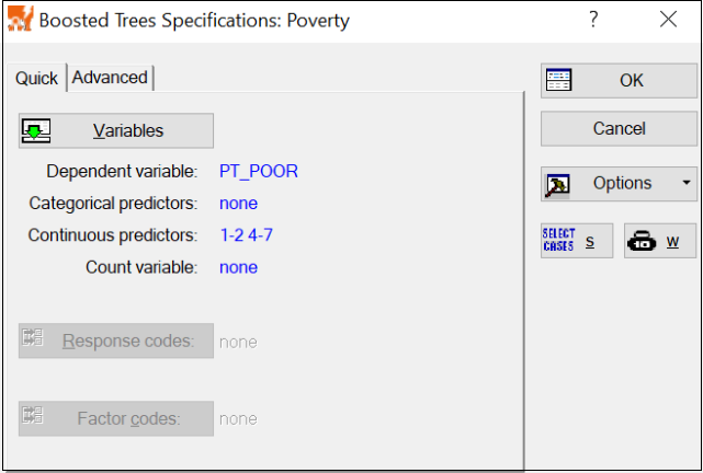
- Select Boosted Tree Classifiers and Regression from the Data Mining menu to display the Boosting Trees Startup Panel. Select Regression Analysis as the Type of analysis from the
Quick tab, and click OK to display the
Boosted Trees Specifications dialog. On the Quick tab, click the Variables button to display the variable selection dialog, select PT_POOR as the dependent variable and all others as the continuous predictor variables, and click the OK button to return to the Specifications dialog.
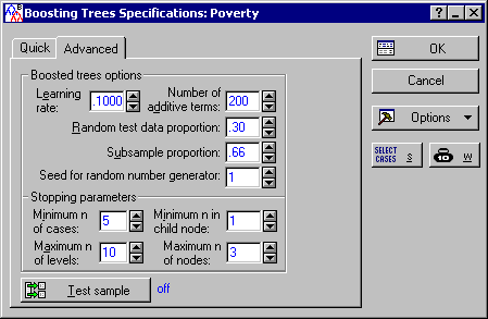
Next, click on the Advanced tab, and set the Subsample proportion to .66.
The Poverty.sta data file is relatively small (with only 30 cases), so we will increase the subsampling rate for the training of each individual tree to a higher (than default) proportion (see also, the Introductory Overview for details).
Now click OK, and after a few seconds the Results dialog will be displayed.
- Reviewing Results
- Click the Summary button on the
Boosting Trees Results dialog - Quick tab to review the average squared error over the successive boosting steps for the training and the testing samples.
In this case, the program chose a relatively simple solution with only 15 additive terms; that was the solution that yielded the smallest Average Squared Error for the Test data.
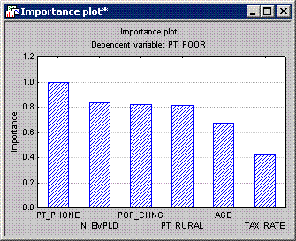
- Predictor importance
- Next click the Bargraph of predictor importance button.
The predictor importance is computed as the relative (scaled) average value of the predictor statistic over all trees and nodes; hence, these values reflect on the strength of the relationship between the predictors and the dependent variable of interest, over the successive boosting steps. As in the analyses performed via the General Classification and Regression Trees module (see Example 2: Regression Tree for Predicting Poverty), variables PT_Phone and N_EMPLD emerge as the most important predictors.
- Plots of predicted and observed values
- Next, select the Prediction tab; here you can select to review various plots of the predicted and residual values to examine how well the current model predicts the dependent variable of interest. In this particular case, the results show that the (few) cases in the testing sample are reasonably well predicted, however, because of the small overall sample size and the differences in the random samples that are created when you follow along with this example, your final solution may look slightly different that was has been reported here.
- Final trees
- You can also review the final sequence of (boosted) trees either graphically or in a sequence of results spreadsheets (one for each tree). However, this may not be a useful way to examine the "meaning" of the final model when the final solution involves a large number of additive terms (simple trees); in this case, the final solution only involves 11 binary trees (each with a simple split). So in this case, it may be useful to review the individual trees in the boosting sequence (in this particular instance, and as expected based on the Barplot of predictor importance, most trees in the boosting sequence describe a simple binary split on variables Pop_Chng, PT_Phone, and N_Empld).
- Deploying the Model for Prediction
- Finally, you can deploy the model (e.g., in a predictive data mining project) via the Code generator on the Results dialog - Report tab. In particular, you may want to save the PMML deployment code for the created model, and then use that code via the Rapid Deployment Engine module to predict new cases (score a data file with new observations).