K-Nearest Neighbor Example 2 - Regression
K-Nearest Neighbor Example 1 is a classification problem, that is, the output was a categorical variable, indicating that the case belongs to one of a number of discrete classes that are present in the dependent variables.
STATISTICA K-Nearest Neighbors (KNN) can be used for solving regression problems where the output is a continuous numeric variable, in which context it acts as a regression technique.
As an example, we will explore the relationship between a single continuous independent variable and a single continuous dependent outcome.
- Data file
- This example is based on the data file Sin250.sta. Open this data file; it is in the /Example/Datasets directory of STATISTICA. The data set consists of two continuous synthetic variables X and Y. The cases of Y are related to X via a simple sin function plus the addition of white (additive) noise.
- Starting the analysis
- Select Machine Learning (Bayesian, Support Vectors, Nearest Neighbor) from the Data Mining menu to display the
Machine Learning Startup Panel.
Select K-Nearest Neighbors on the Quick tab, and click the OK button to display the K-nearest neighbors dialog. You can also double-click on K-Nearest Neighbors to display this dialog.
- Analysis settings
- On the
Quick tab, click the Variables button to display a standard variable selection dialog. Select Y as the Continuous dependent variable and X as the Continuous predictor (independent) variable, and click the OK button.
At this stage, you can change the settings for your analysis, e.g., the sampling technique (see the documentation for the Sampling tab) for dividing the data into examples and test samples, and the number of nearest neighbors K, as well as the distance measure (metric) and the averaging scheme (see the documentation for the Options tab). For analyses with more than one independent variable with significantly different typical values, you may also want to standardize the distances (for continuous independent variables only). For further details see below. The significance of the averaging scheme is also discussed below.
One important setting to consider is the sampling technique for dividing the data into examples and testing samples (on the Sampling tab). For more details, see the documentation for the K-Nearest Neighbors dialog - Sampling tab.
When performing KNN analyses, it is recommended that you standardize the independent variables so that their typical case values fall into the same range. This will prevent independent variables with typically large values from biasing predictions. To apply this scaling, on the K-nearest neighbors dialog - Options tab, select the Standardize distances check box (this option is also available on the Results dialog). However, for the current example this is not necessary since the data set consists of only one independent variable.
Now, display the Cross-validation tab. Select the Apply v-fold cross-validation check box, and increase the Maximum number of nearest neighbors to 20.
Now, click the OK button. While KNN is searching for an estimate of K using the cross-validation algorithm, a progress bar is displayed followed by the K-Nearest Neighbor Results dialog.
- Reviewing results
- On the
K-Nearest Neighbors Results dialog, you can perform KNN predictions and review the results in the form of spreadsheets, reports, and/or graphs.
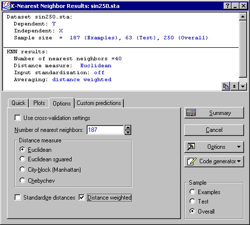
In the Summary box at the top of the Results dialog, you can see some of the specifications of the KNN analysis, including the list of variables selected for the analysis and the size of example, test, and overall samples (when applicable). Also displayed are the number of K nearest neighbors, distance measure, and whether input standardization and weighting based on distance are in use. You can also review the cross-validation error. Note that these are specifications that were made in the K-nearest neighbors dialog, displayed here for your reference.
On the Quick tab of the Results dialog, click the Cross-validation error button to create the graph of the cross-validation error for each value of K tried by the cross-validation algorithm.
The first thing you should look for in this graph is the existence of a saddle point, i.e., a value of K with minimum error compared to its neighboring points. The existence of a minimum indicates that the search range for K was sufficiently wide to include the optimal (from a cross-validation sense) value. If it is not present, return to the KNN dialog by clicking the Cancel button on the Results dialog, and increase the search range.
As discussed before, STATISTICA KNN makes predictions on the basis of a subset known as examples (or instances). Click the Model button to create a spreadsheet containing the case values for this particular sample.
Further information on the regression analysis can be obtained by clicking the Descriptive statistics button to create a spreadsheet containing various regression statistics including the S.D. ratio and the correlation coefficient between the observed and predicted values.
Also, you can display the spreadsheet of predictions (and include any other variables that might be of interest to you, e.g., independents, dependents, residuals, etc., by selecting the respective check boxes in the Include group box) by clicking the Predictions button.
You can display these variables in the form of histogram plots by clicking the Histograms button.
Further graphical review of the results can be made by selecting the Plots tab and creating two- and three-dimensional plots of the variables, predictions, and their residuals. Note that you can display more than one variable in two-dimensional scatterplots.
For example, shown below is a scatterplot of the predicted and observed values of Y plotted against the values in the variable X. In general, this type of plot will give you an effective way of comparing model predictions with the observed data. To produce this graph, on the Plots tab, select the Test option button in the Sample group box, select X in the X-axis list, and select Observed and Predicted in the Y-axis list. Then click the Graphs of X and Y button.
Note: you can determine the sample (subset) for which you want to display the results. Do this by making a selection from the Sample group box on the K-Nearest Neighbors Results dialog. For example, select the Overall option button to include both the examples and test samples in spreadsheets and graphs. However, note that you cannot make predictions (and other related variables, e.g., accuracy or confidence) for the examples sample since it is used by KNN for predicting the testing sample. The following spreadsheet was created by clicking the Predictions button on the Quick tab.Since there is no model fitting in a KNN analysis, the results you can produce from the Results dialog are by no means restricted to the specifications made on the K-nearest neighbors dialog. To demonstrate this, select the Options tab of the Results dialog, and clear the Use cross-validation settings check box. This will enable the rest of the controls on this tab, which are otherwise unavailable. (Note: This action will not discard the cross-validation results. You can always re-set your analysis to this setting by selecting the check box again). Change the number of nearest neighbors to 40.
On the Plots tab, select the independent variable X as the X-axis, and Observed and Predicted as the Y-axis. Click the Graph of X and Y button to produce the graph of X against the Observed and Predicted values of the independent variable Y. Note that due to the larger value of K (compared to the cross-validation estimate 5) predictions have already started to deteriorate (KNN misses its targets on both sides of the regression curve).
At this point, you may want to display a new descriptive statistics spreadsheet (from the Quick tab) from which you will note a decrease in the model variance. Indeed, the variance will continue to diminish with the increase in K.
When K is as large as the size of the examples sample (k=187; i.e. enter 187 in the Number of nearest neighbors field on the options tab) the model variance becomes zero and the regression curve is now a constant line (which is simply the average value of the dependent variable Y).
Next, let's study the effect of distance weighting on KNN predictions. On the K-Nearest Neighbors Results dialog - Options tab, select the Distance weighted check box, and clear the Standardize distances check box. Leave K at 187.
and produce the graph of X against the observed and predicted value of Y. Note the difference between this graph and the previous one.
Finally, select the Custom predictions tab in order to perform a "what if?" analysis. Using the options on this tab, you can define new cases (that are not drawn from the data set) and execute the KNN model. This enables you to perform ad. hoc. "What if?" analyses. Click the Predictions button to create the prediction of the model.