Example 9.2: Mixture Designs for Components with Upper and Lower Bound Restrictions
- Overview
- A very common application of the facilities for finding vertex and centroid points is in the context of mixture designs when the component values are restricted by both upper and lower bounds. (Mixture designs, where the sum of the component values must be constant, are discussed in detail in the Introductory Overview, see also
Example 8.1 and
Example 8.2.) For example, Cornell (1990a) describes a mixture design problem concerned with the formulation of vinyl as used for automobile seat covers. Three plasticizers (A, B, and C) make up most of the mixture, and their proportions are restricted by the following constraints.
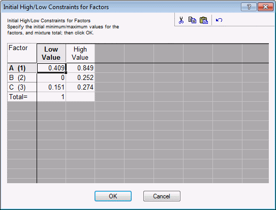
.409 < xA < .849
0 < xB < .252
.151 < xC < .274
Example 8.2 describes how to construct standard mixture designs in pseudo-components, that is, in a sub-simplex defined by the lower-bound constraints for the components. When both lower and upper bound constraints are present for some or all of the components, the standard designs can no longer be constructed.
As an alternative, we can find the vertex and centroid points of the experimental region (inside the simplex or triangle) defined by the constraints, and then select from those the points for the final experiment.
- Specifying the constraints
- After starting the Experimental Design module, in the Startup Panel, select the Advanced tab. Double-click Designs for constrained surfaces and mixtures to display the
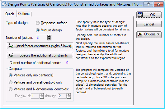
Design Points (Vertices & Centroids) for Constrained Surfaces and Mixtures dialog box. Then select Mixture design as the Type of design.
Next, click the Initial factor constraints (highs & lows) button, and specify the high and low component settings in the Initial High/Low Constraints for Factors dialog box as shown below.
Click OK to accept these values.
The constraints in this example pertain entirely to the upper and lower bound restrictions on the components. However, note that other, additional (linear) constraints could also be handled. In this example, there are no additional constraints.
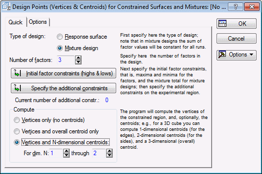
In the Compute group box, select the Vertices and N-dimensional centroids option button so that the centroid points are also computed. The dialog box should now look as shown below.
- Reviewing results
- Click OK to display the
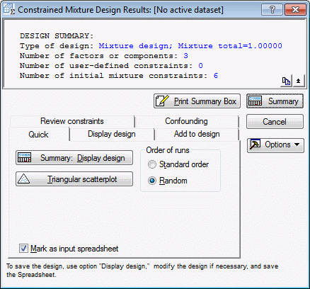
Constrained Mixture Design Results dialog box.
The quickest way to visualize the constrained region is in a scatterplot of the vertex and centroid points; since this is a mixture design, a Triangular scatterplot will be produced (see the Introductory Overview, for an explanation of these plots).
Select the Review constraints tab, clear the Plot vertex points only check box, and click the Triangular scatterplot button. The valid experimental region is defined by a small area inside the full triangle (see also Cornell, 1990a, Figure 14).
Now, on the Quick tab, click the Summary: Display design button (shown below in Standard order).
- Analyzing the design
- Close all results and dialog boxes.
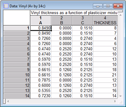
Cornell (1990a, Table 13) constructed from these 9 points a 14-run experiment (by replicating the vertex points, and the overall centroid, labeled C(2) in the spreadsheet shown above).
The data for the completed experiment are contained in the example data file Vinyl.sta. Open this data file.
The analysis of these data can proceed exactly in the same way as described for standard mixture designs (see Example 8.1) or for mixture designs with lower-bound constraints (see Example 8.2:).
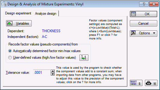
Start Experimental Design (DOE). In the Design & Analysis of Experiments Startup Panel, select Mixture designs and triangular surfaces and click the OK button.
In the Design & Analysis of Mixture Experiments dialog box, select the Analyze design tab.
Click the Variables button, and in the variable selection dialog box, specify Thickness as the Dependent variable and A, B, and C as the Independent vars (factors). Click OK in the variable selection dialog box
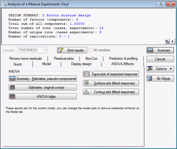
Click OK to proceed to the Analysis of a Mixture Experiment dialog box.
Cornell (1990a) fits to these data the quadratic model; therefore, select the Model tab, and select the Quadratic option button.
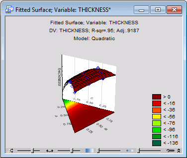
To see the constrained surface, select the Quick tab and click the Surface plot (fitted response) button.
You can use the Interactive Graphics Controls at the bottom of the graph window to rotate the graph and/or adjust the transparency of the plot areas to view different aspects of the plot.
As explained in Example 8.2 and the Introductory Overview, this plot shows the fitted surface for the pseudo-components, to provide better "resolution" for the fitted surface.
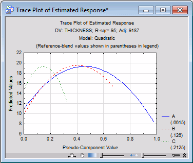
Now click the Trace plot of expected response button. In the Values for Reference Blend dialog box, .6615, .126, and .2125 should be displayed (which is approximately the center for the pseudo-components). Click OK to produce the graph.
We can clearly see that component C has a very narrow valid range, but its precise setting appears to be important, as indicated by the strongly curved response trace.
Note that, in order to see the original constrained region, you can force the program not to use the pseudo-component transformation (see Example 8.2).
To rerun the analysis, click Cancel in the Analysis of a Mixture Experiment dialog box to return to the Design & Analysis of Mixture Experiments dialog box.
In the Recode factor values (pseudo-components) from group box, select the User-defined values (high/low factor values) option button, which will display the Specifications for Mixture Variables dialog box.
Click OK to accept the default factor highs and lows (1 and 0, respectively) for the pseudo-component transformation.
Click OK in the Design & Analysis of Mixture Experiments dialog box to display the Analysis of a Mixture Experiment dialog box.
On the Model tab, select the Quadratic option button, and on the Quick tab, click the Surface plot (fitted response) button to show the second-order surface fitted to the original components.
As mentioned in Example 8.2, the overall conclusions from the experiment are not affected by analyzing pseudo-components or original component values, because the pseudo-component transformation is linear.
See also, Experimental Design.

