Naive Bayes Classifier Example - Classification

For the example, we will use the classic Iris data set. This data set contains information about three different types of Iris flowers: Versicolor, Virginic, and Setosa. The data set contains measurements of four variables [sepal length and width (SLENGTH and SWIDTH) and petal length and width (PLENGTH and PWIDTH)]. The Iris data set has a number of interesting features:

Data file

Open the IrisSNN.sta data file; it is in the /Example/Datasets directory of STATISTICA.

Starting the analysis

Select Machine Learning (Bayesian, Support Vectors, Nearest Neighbor) from the Data Mining menu to display the Machine Learning Startup Panel.

Select Naive Bayes Classifiers on the Quick tab, and click the OK button to display the Naive Bayes dialog. You can also double-click on Naive Bayes Classifiers to display this dialog.

Analysis settings

On the Quick tab, click the Variables button to display a standard variable selection dialog, select FLOWER as the Categorical dependent variable and variables 2-5 as the Continuous predictors (independent) variable list, and click the OK button.

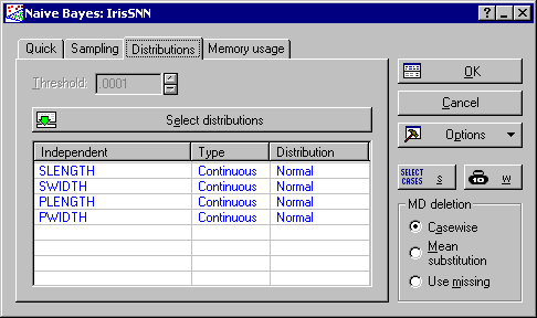
At this stage, you can change the specifications of the analysis, e.g., the sampling technique for dividing the data into train and test samples (Sampling tab), and the threshold and the distribution of the continuous inputs (Distributions tab). Note that the threshold imposes a lower bound on the conditional probability of an input categorical level given an output class. Thus, this option is only available when categorical inputs are present in your analysis.

One important setting to consider is the sampling technique for dividing the data into examples and testing samples (on the Sampling tab). Although the choice of a sampling variable is not the default setting (as a  sampling variable may not be available in your data set) you may want to use this option since it divides the data deterministically, unlike random sampling. Using a sampling variable enables you to compare  various results with different experimental settings. It is always recommended that you provide a test sample as an independent check on the performance of your model.

The default distribution for the continuous independent variable is normal.

You can change this option in a way that suits the statistical properties of your data set; e.g., if you believe that the distribution of a certain independent variable is better represented by a lognormal, assign this type of distribution to the variable in question. To do this, display the Distributions tab and click the Select distributions button. A standard variable selection dialog will be displayed, which you can use to assign distributions of your choice to the continuous independent variables. For most problems, however, the default choice of a normal input distribution is desired.

Because of the nature of Naive Bayes classifiers, you can make use of data cases that are partially valid, i.e., data cases with both valid and missing or invalid entries. Consider the following data case for example:

Inputs = {0.14  0.23  MISSING  4.6  MISSING}, output = {Setosa}

Although some of the entries are missing, this data case can still be used in building the Naive Bayes model. For example, you can use the entry Setosa in computing the prior probabilities of class membership. Equally, you can use a valid independent entry to estimate the parameters of the corresponding distribution. This method is particularly useful when the data set is sparse, i.e., data sets with a substantial number of missing entries.

To specify this in our example, select the Use missing option button in the MD deletion group box in the Naive Bayes dialog.

Reviewing results

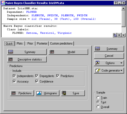
Now click the OK button on the Naive Bayes dialog to display the Naive Bayes Classifier Results dialog, where you can create results in the form of spreadsheets, reports, and/or graphs.

In the Summary box at the top of the Results dialog, you can view specifications that were made in the Naive Bayes dialog, including the dependent and independent variable list and the number of valid data cases in each sample. You can also view the dependent variable and its class labels.

Naïve Bayes constructs the decision function using a set of conditional probabilities for the independent variables. These probabilities are then combined to form a likelihood, which in turn is combined with the class prior probability, using Bayes' rule, to form the final posterior. The posterior forms the basis of the decision function.

Click the Model button (on the Quick tab) to create a spreadsheet of the Naïve Bayes model for each dependent variable.

This spreadsheet contains full details of the conditional and prior probabilities for the class variables. This is useful for a detailed review of the Naive Bayes model you have constructed or for inclusion in your reports.

Further information can be obtained by clicking the Descriptive statistics button, which will display a spreadsheet of classification summary and a confusion matrix for each dependent variable (note that Naive Bayes can compute multiple dependent variables).

Using these spreadsheets, you can view the rates of correctly and misclassified cases. Note that you can produce these spreadsheets for Training, Testing, or Overall samples by selecting the respective option in the Sample group box of the Results dialog.

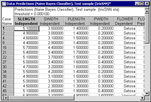
To further view results, you can display the spreadsheet of predictions (and include any other variable that might be of interest to you, e.g., independent, dependents, accuracy, etc.). You can also display these quantities as histogram plots.

To generate a predictions spreadsheet, select all the check boxes in the Include group box of the Naive Bayes Classifier Results dialog - Quick tab.

Now, click the Predictions button.

A close inspection of this spreadsheet indicates that class Setosa is completely separable from Versicol and Virginic, while the latter two display a noticeable degree of overlapping (confusion). This can be observed from the incorrectly classified cases, which happen to belong to Versicol. A further look at the confidence levels will also confirm this finding. Note that the Naive Bayes model classifies Setosa with probability 1 (i.e., %100 confidence) when cases truly belong to Setosa. Note that this is not the case for Versicol and Virginic.

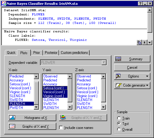
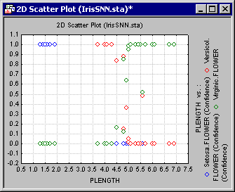
To view this effect and the overlapping of the class labels, select the Plots tab and specify PLENGTH (for example) as the X-axis and Setosa ( conf.), Versicol ( conf.), and Virginic ( conf.) as the Y-axis.

Then click the Graphs of X and Y button.

From the generated graph, note the high levels of confidence that Setosa is achieving when the case labels truly belong to this categorical level. Compare this to Versicol and Virginic, for which there is a significant degree of overlap (i.e., having similar confidence) between them, which coincides with the area where PLENGTH~4.5. It is in this region where misclassification occurs.

Further graphical review of the results can be made by creating two- and three-dimensional plots of the variables, predictions, and accuracy. As demonstrated above, you can display more than one variable in two-dimensional scatterplots.

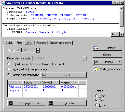
Next, we'll demonstrate the effect of the designated class priors probabilities on predictions. Click on the Prior tab and select the Custom prior probability option button. Click the Select button to display the Specify prior values dialog. Change the prior values for the class variables to match the following: Setosa = 0.5, Versicol = 0.5, and Virginic = 0.0. Click the OK button to confirm the changes and return to the Results dialog.

Next, click the Predictions button (on the Quick tab) to create the predictions spreadsheet.

Compare this new spreadsheet with the previous ones, and you will note that cases belonging to Virginic are now misclassified as Versicol. This is because the prior for Virginic was set to zero, which forbids classifying cases with that particular categorical level. This example, however, was an extreme case, i.e., one of the class variables was set to zero. More generally, a large prior will encourage independent cases to be classified with the associate categorical level, while alternatively a small prior will discourage identifying cases as such. Thus, prior values need to be carefully chosen when using Naive Bayes.

On the Prior tab, select the Default Prior Probability option button to re-set the priors to the default values (i.e., base their values on the frequency of the class labels found in the training data).

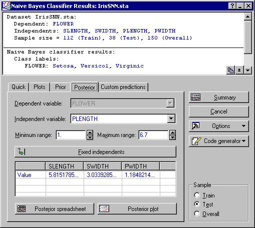
Now let's investigate the effect of adjusting an independent variable on the confidence levels (and, hence, predictions) using the Posterior tab. While one specially chosen numeric independent variable is altered (and plotted across the x-axis of the graph), values must also be provided for the other variables. These are given fixed values, and are referred to as Fixed independents.

In the Independent variable field, select PLENGTH from the drop-down list.

Accepting all defaults, click the Posterior plot button to create a line plot of the confidence levels. You can repeat the above steps for various settings and compare the results.

Finally, you can perform a "what if?" analysis using the options on the Custom predictions tab. Define new cases (that are not drawn from the data set) and execute them using the Naive Bayes model, which enables you to perform ad-hoc, "What if?" analyses. The prediction of the model can be displayed (together with the independent cases) by clicking the Predictions button, but first click the User defined case button to display a general user entry spreadsheet.

Use this spreadsheet to enter values for the independent variables, as shown in the above illustration. Click OK to confirm the new entries and return to the Results dialog. Then, click the Predictions button to create a spreadsheet containing the new independent cases and the Naive Bayes response.