Example 3: A 2-Level Between-Group x 4-Level Within-Subject Repeated Measures Design
- Overview
-
This example demonstrates how to set up a repeated measures design. The use of the post-hoc testing facilities will be demonstrated, and a graphical summary of the results will be produced. Moreover, the univariate and multivariate tests will be computed.
Research Problem
This example is based on a (fictitious) data set reported in Winer, Brown, and Michels (1991, Table 7.7). Suppose we are interested in learning how different factors affect people's ability to perform a fine-tuning task. For example, operators of complex industrial machinery constantly need to read (and process) various gauges and adjust machines (dials) accordingly. In this (fictitious) study, two methods for calibrating dials were examined, and each subject was tested with 4 different shapes of dials.The resulting design is a 2 (Factor A: Method of calibration; with 2 levels) by 4 (Factor B: Four different shapes of dials) analysis of variance. The last factor is a within-subject or repeated measures factor because it represents repeated measurements on the same subjects; the first factor is a between-groups factor because subjects will be randomly assigned to work under one or the other Method condition.
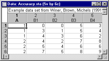
- Data file
- The setup of a data file for repeated measures analysis is straightforward: The between-groups factor (A: Method of calibration) can be specified by setting up a variable containing the codes that uniquely identify to which experimental condition each subject belongs. Each repeated measurement is then put into a different variable. Shown below is an illustration of the data file Accuracy.sta.
- Specifying the Design
- Open the Accuracy.sta data set, and start the
General ANOVA/MANOVA analysis.
Following are instructions to do this from the ribbon bar and from the classic menus.
Ribbon bar. Select the Home tab. In the File group, click the Open arrow and from the menu, select Open Examples to display the Open a STATISTICA Data File dialog box. Double-click the Datasets folder, and then open the Accuracy.sta data set.
Next, select the Statistics tab. In the Base group, click ANOVA to display the General ANOVA/MANOVA Startup Panel.
Classic menus. Open the data file by selecting Open Examples from the File menu to display the Open a STATISTICA Data File dialog. The data file is located in the Datasets folder.
Then, from the Statistics menu, select ANOVA to display the General ANOVA/MANOVA Startup Panel.
In the Startup Panel, select Repeated measures ANOVA as the Type of analysis and Quick specs dialog as the Specification method, and then click the OK button (see the Introductory Overview for different methods of specifying designs). In the ANOVA/MANOVA Repeated Measures dialog, click the Variables button to display the standard variable selection dialog. In the Dependent variable list select B1 through B4; in the Categorical predictors (factors) list, select A. Click the OK button. Next, click the Factor codes button to display the Select codes for indep. vars (factors) dialog. Click the All button to select the codes (1 and 2) for the independent variable, and click the OK button to close this dialog and return to the ANOVA/MANOVA Repeated Measures dialog.
- Specifying the repeated measures factors
- Next click the Within effects button to display the
Specify within-subjects factor dialog. Name the repeated measures factor B (in the Factor Name box) and specify 4 as the No. of levels. When reading the data, STATISTICA will go through the list of dependent variables and assign them to represent the consecutive levels of the repeated measures factor. See
General ANOVA/MANOVA and GLM Notes - Specifying Within-Subjects Univariate and Multivariate Designs for more information on how to specify repeated measures factors.
Now click the OK button to close this dialog, and click the OK button in the ANOVA/MANOVA Repeated Measures dialog to run the analysis and display the ANOVA Results dialog.
- Reviewing Results
- The
Results dialog contains options for examining the results of the experiment in great detail.
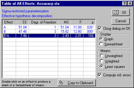
Let's first look at the summary table of All effects/Graphs (click the All effects/Graphs button on the Quick tab).
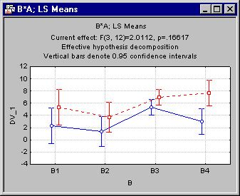
Select Effect B*A as shown above (even though this effect is not statistically significant), and click the OK button; also click OK in response to the prompt about the assignment of factors to aspects of the graph (i.e., accept the defaults in the Arrangement of Factors dialog).
It is apparent that the pattern of means across the levels of the repeated measures factor B is approximately the same in the two conditions A1 and A2. However, it appears that there is a particularly strong difference between the two methods for dial B4, where the confidence bars for the means do not overlap.
- Planned Comparison
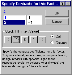
- Next, let's examine the differences between the means for B4. Click on the
Comps (comparisons) tab, and then click the Contrasts for LS means button to specify the contrasts for least squares means. Note that the so-called least squares means represent the best estimate of the population means mu, given our current model; hence, STATISTICA performs the planned comparison contrasts based on the least squares means; however, in this case it is not so important since this is a complete design where the least squares means are usually identical to the observed means.
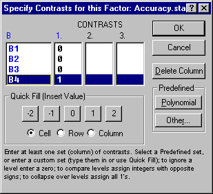
We are interested in comparing method A1 with method A2, for dial B4 only. So, in the Specify Contrasts for this Factor dialog, for specifying the contrast for factor A, set the contrast coefficients as shown below:
Click the OK button and on the larger Specify Contrasts for this Factor dialog, set all coefficients to 0 (to ignore the respective means in the comparison), except for B4.
Refer to General ANOVA/MANOVA and GLM Notes - Specifying Univariate and Multivariate Between-Groups Designs for additional details on the logic of testing planned comparisons.
Now click the OK button, and click the Compute button on the Comps tab. Here are the results.
It appears that, as was evident in the plot of means earlier, the two means are significantly different from each other.
- Post-Hoc Testing
- Since we did not have a priori hypotheses about the pattern of means in this experiment, the a priori contrast, based on our examination of the pattern of means is not "fair." As described in the Introductory Overview, the planned comparison method capitalizes on chance when you only compare those means that happen to be most different (in a study of, for example, 2*4=8 means, such as in this study).
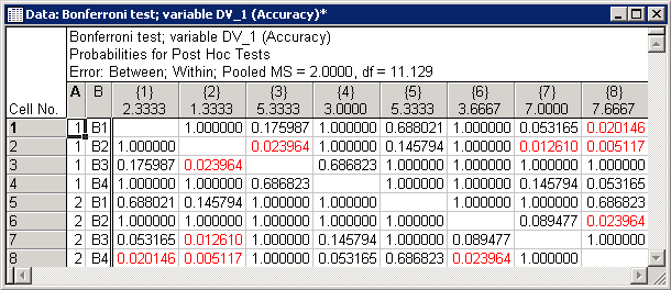
To compute post-hoc tests, click the More results button to display the larger and more comprehensive Results dialog. Click on the Post-hoc tab, select effect B*A (i.e., the B by A interaction effect) in the Effect box, select the Significant differences option button as the display format in the Display group, and then click the Bonferroni button.
As you can see, using this more conservative method for testing the statistical significance of differences between means, the two B4 dials, across the levels of A are not reliably different from each other.
The post-hoc tests are further explained in the Post-hoc tests in GLM, GRM, and ANOVA topic; note also that when testing means in an interaction effect of between-group and within-subject (repeated measures) effects, there are several ways (options in STATISTICA) to estimate the proper error term for the comparison. These issues are discussed in Error Term for Post-hoc Tests in GLM, GRM, and ANOVA; see also Winer, Brown, and Michel (1991, p. 529-531) for a discussion of the Pooled MS reported in this results spreadsheet.
- Tests for the B main effect
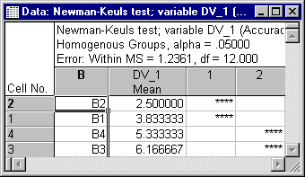
- Winer, Brown, and Michels (1991, Table 7.10) summarize the results of using the Newman-Keuls procedure for testing the differences in the B main effect. To compute those tests, on the
Post-hoc tab, select as the Effect the B main effect, then select the Homogeneous groups option button under Display, and then click the Newman-Keuls button.
In this table, the means are sorted from smallest to largest, and the means that are not significantly different from each other have four "stars" (*) in the same column (i.e., they form a homogenous group of means); all means that do not share stars in the same column are significantly different from each other. Thus, and as discussed in Winer, Brown, and Michels (1991, p. 528), the only means that are significantly different from each other are the means for B2 vs. B4 and B3, and B1 from B4 and B3.
- Multivariate Approach
- In the Introductory Overview and
Notes, the special assumptions of univariate repeated measures ANOVA were discussed. In some scientific disciplines, the multivariate approach to repeated measures ANOVA with more than two levels has quickly become the only accepted way of analyzing these types of designs. This is because the multivariate approach does not rest on the assumption of sphericity or compound symmetry (see Assumptions - Sphericity and Compound Symmetry).
In short, univariate repeated measures ANOVA assumes that the changes across levels are uncorrelated across subjects. This assumption is highly suspect in most cases. In the present example, it is quite conceivable that subjects who improved a lot from time (dial) 1 to time (dial) 2 reached a ceiling in their accuracy, and improved less from time (dial) 2 to time (dial) 3 or 4. Given the suspicion that the sphericity assumption for univariate ANOVA has been violated, look at the multivariate statistics.
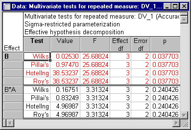
On the Summary tab, select all types of Multivariate tests (select all of the check boxes under Multivariate tests), and then click the Multiv. tests button under Within effects.
In this case, the same effect (B) is still statistically significant. Note that you can also apply the Greenhouse-Geisser and Huynh-Feldt corrections in this case without changing this pattern of results (see also Summary Results for Within Effects in GLM and ANOVA for a discussion of these tests).
- Summary
- To summarize, these analyses suggest that both factors A (Method) and B (Dials) significantly contributed to subjects' accuracy. No evidence was found for any interaction between the two factors.