If you want to create an interactive scatterplot, you can use the
scatterplot3js function from the threejs package.
About this task
You can use RStudio
to create this 100,000-point interactive scatter plot, or you can use the
TERR
console and display the results in a browser.
Before you begin
TERR, access to the internet, and a browser.
Procedure
-
From the TERR console or RStudio
prompt,
install the threejs package.
install.packages("threejs")
TERR checks TRAN and then CRAN for
the packages to install, and then installs them along with any packages they
require.
-
Call the
library function to load the required packages.
-
Assign the value
10000 to
N1, and the value
90000 to the name
N2.
-
Assign the point distribution to the
x axis.
Set a random normal distribution for both
N1 and
N2, with the standard deviation for
N1 of
.05, and the standard deviation for
N2 of
2.
x <- c(rnorm(N1, sd=0.5), rnorm(N2, sd=2))
-
Assign the point distribution to the
y axis.
Set a random normal distribution for both
N1 and
N2, with the standard deviation for
N1 set to
.05, and the standard deviation for
N2 set to
2.
y <- c(rnorm(N1, sd=0.5), rnorm(N2, sd=2))
-
Assign the point distribution to the
z axis.
Set a random normal distribution for
N1, with the standard deviation of
.05, and a random Poisson distribution for
N2 with lambda of
20 to specify the means. Subtract 20 from the
concatenation to center the points correctly on the
z axis.
z <- c(rnorm(N1, sd=0.5), rpois(N2, lambda=20)-20)
-
Assign to
col the color values for
N1 and
N2.
Set
N1 points to be yellow (#ffff00)
and set the
N2 points to be blue (#0000ff).
col <- c(rep("#ffff00",N1),rep("#0000ff",N2))
-
Call the threejs function
scatterplot3js to create the three-dimensional plot.
Plot the points for the coordinate values
x,
y, and
z axes in the three-dimensional graph, setting the
colors to
col, and the point size to
0.25.
scatterplot3js(x,y,z, color=col, size=0.25)
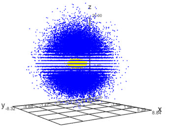
Results
A browser opens and
shows the three-dimensional scatterplot, which you can reposition to see the
point distribution.
Tip: Dragging
the visualization vertically reveals the
N1 points centered in the cloud of
N2 points.