NLP Use Case

Mac versus PC Article Classification

For our use case, we began with a folder of articles about Macintosh hardware and a folder of articles about IBM PC hardware. We built a classifier that could determine whether a new article is posted by the Mac user group or the PC user group.

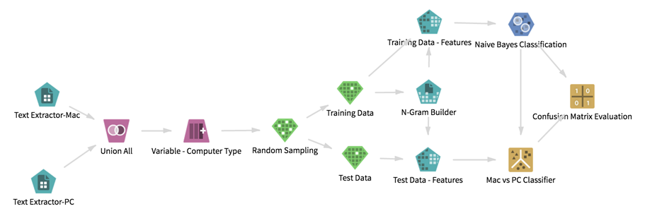
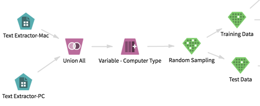
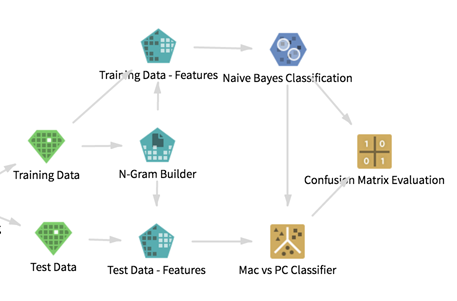
Below is the resulting workflow. In this article, we describe how we built the workflow to get meaningful information.

Datasets

The data came from the 20 Newsgroups Dataset, which contains messages from popular Usenet groups. We used text from two newsgroup folders.

Each of these folders contained 1000 text files, each of which contained one message. The data was in plain text format. We parsed out the relevant information using the available NLP operators.

To download the data, we browsed to the Twenty Newsgroups page and clicked Download Data Folder to download the .tar.gz file, and then extracted it to a folder.

Workflow

Load the Data to HDFS

The data must be in HDFS to be accessible to Team Studio. To add the data, we connected to the cluster using SSH, and then copied the folder containing the text files into a location accessible by Team Studio.

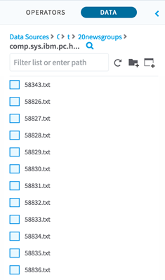
In the data source, we named one folder comp.sys.mac.hardware and we named a second folder comp.sys.ibm.pc.hardware. Each folder contained the 1000 files of the form <number>.txt:

Data Cleaning

We put our imported text data into a tabular format, and then generated features for the classification.

The cleaned data needed to have the following fields.

• The computer_type categorical variable, which is used to indicate whether the message is from the Mac group or the PC group.
• Numeric features (from the NLP operators) such as n-gram counts, which are passed to Team Studio classification operators.

To train different models, we created two random samples from the dataset. One sample is the training set, and the other sample is the test set.

The data transformation procedure is as follows.

1. We used the Text Extractor operator on both of the folders. This operation consolidated the messages in each folder into one dataset, with one row per article. The resulting dataset included several columns about the parsing process.

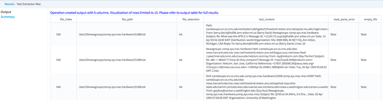
   For example, we ran the text extractor on the comp.sys.mac.hardware directory to get the following output.

   
   
   

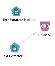
   The operator includes columns with the file index, path, extension, the content of the article, and any errors associated with parsing. (This example focuses on file_path and text_content for the analysis.)

   Note: The operator does not fail if some of the documents are malformed, but malformed documents are not included in the analysis.
2. The data was now in two datasets, but we needed it to be in just one dataset. To accomplish this, we used the Set Operations operator.

   We needed to retain the information about whether a message is from the Mac group or the PC group. The documents had already been classified into two folders. We could preserve the information about the classification by leaving them in the two folders and running the Text Extractor operator on each of the two folders separately. Then we could use the Union All setting in the Set Operations to combine the data from both folders. (We named the operator Union All for clarification purposes.)

   
   
   

3. With the data now in one file, we extracted the computer type from the newsgroup path and tagged it with the easier-to-read computer_type variable using a Pig expression in the Variable operator.

   Remember that the two newsgroups are named comp.sys.mac.hardware and comp.sys.ibm.hardware. We care only about the mac and ibm part of the file path. To extract that part, we used the Pig expression SUBSTRING(file_path,28,31)

   Tip: You can use Team Studio to design a similar ETL process. In this example, articles all in the same folder can have names that represent their types (for example, Mac_1.txt), or you can join a dataset with the path and some metadata about each article to the output of the Text Featurizer.
4. We used the Random Sampling operator to break the data into two samples: the training sample and the test sample. We split our samples into 80% for our training sample and 20% for our test sample.
5. We used two Sample Selector operators to split out random samples into the training set and the test set. We connected the Random Sampling operator to our two Sample Selector operators to achieve this.

   At this point, our workflow looked like the following. It was ready to apply the model.

   
   
   

Modeling

We used the training and test sets to create some features from the data using NLP operators, and then we ran a classification and confusion matrix to see how well the model performed.

1. On the training data, we used the N-Gram Dictionary Builder to create a dictionary of words used to create the features. We specified tokenization and parsing options. The dictionary builder creates a dictionary of the n-grams (words or phrases) in the training corpus. When you featurize a dataset for either training a model or predicting, you must use the same N-gram Dictionary Builder to ensure that you are creating features from the same n-grams.

   The N-gram Dictionary Builder also defines how to tokenize the document. This tokenization must also be consistent across the training and test data. You can learn more about the configuration options for the N-gram Dictionary Builder in its help topic, but in this use case, we used default options.

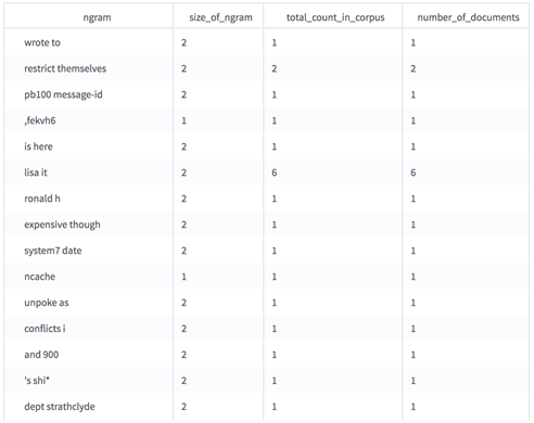
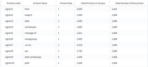
   The output of the N-gram Dictionary Builder displays all the n-grams in all the documents, how frequently those n-grams appear, and in how many documents they appear.

   
   
   

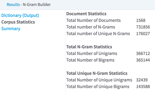
   It also conveys statistics about all of the documents.

   
   
   

   The N-gram Dictionary Builder cannot be connected to Team Studio operators other than the Text Featurizer. However, it does write tabular output to HDFS. To use this output, navigate to the location you specified to store the results, and then drag that result file onto the workflow canvas. (Another example of something you could do with the dictionary results here is run it through a sorting operator to see which n-grams appeared in the most documents.)

2. We used the Text Featurizer operator to select the most commonly used 500 words from the dictionary. Then, for each message, we scored how many times each word appeared.
   To provide features for both the training set and the test set, we did the following.

   1. Connected a Text Featurizer operator to both the training data and the N-Gram Dictionary Builder.
   2. Connected a Text Featurizer operator to the test data and the N-Gram Dictionary Builder.
   3. Configured each operator with the following settings:

   Setting	Configuration
   Text Column	text_content
   N-Gram Selection Method	Appear in the Most Documents
   Maximum Number of Unique N-grams to Select (or Feature Hashing Size)	500
   For Each N-Gram and Document Calculate	Normalized N-Gram Count
   Use N-Gram Values as Column Names	No
   Storage Format	CSV
   Output Directory	@default_tempdir/tsds_out
   Output Name	@operator_name_uuid
   Overwrite Output	true
   Advanced Spark Settings Automatic Optimization	Yes

   For each tokenized article, we counted the number of times each of the 500 selected n-grams appeared, and then normalized the counts against the number of tokens in the document. Thus, we computed a metric of how frequently the word appeared relative to the length of the article. By selecting the computer_type column in the Columns To Keep field, we used it as the dependent variable in the classification algorithms.

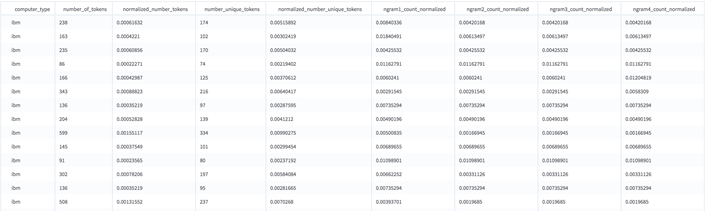
   The result of each Text Featurizer is a dataset where each row represents one article, and each column is a numeric feature.

   The first column(s) are the columns from the original dataset we selected to keep. In this case, we selected to keep only one: the computer_type column. The next four columns contain some generic statistics about each article.

   • number_of_tokens - the number of tokens (words) in the article.
   • normalized_number_tokens - the number of tokens in the article, normalized against the average number of tokens in the all of the articles.
   • number_unique_tokens - the number of unique words in the article.
   • normalize_number_unique_tokens - the above, normalized against the average of the corpus.

   
   
   

   The next 500 columns each represent the normalized count of one of the most commonly used n-grams. ngram1_count_normalized is the normalized count per document of the most common n-gram in the training corpus.

   ngram1 is still unknown. To find out what it is, we looked at the N-Grams to Column Names section of the results.

   For this example, note that ngram1 is the token from.

   
   
   

   Now we had a dataset with numeric columns that represent the frequency of the n-grams in each document, and one categorical column with the category of that document. This example uses the simplest classification algorithms, but now we can integrate the text data with nearly all of the analytic power of Team Studio. We can apply any of the Team Studio transformation operators to further clean and process the data. We can explore the content of the corpus using the exploration operators, such as Summary Statistics. We can cluster the documents into new, previously unknown categories. We can see if the presence of some n-grams depends on others with any of the regression algorithms. We can even build a Touchpoint on top of the trained classification algorithm to classify new documents.

3. Naive Bayes is one of the most common algorithms used for text classification. We applied Naive Bayes to the featurized dataset, building a classifier that can classify a new document as either from the Mac or IBM user group.

   We connected the featurized dataset to the Naive Bayes operator, and then we used the document category as the dependent column and the text features (for example, Ngram1_normalize_count) or (Doc_count) as independent variables.

   Optionally, we could export this model using Export. Instead, we used it in a workflow to predict the subject of new documents.

Predicting and Classifying

To use a predictor or a classifier with NLP data, you must clean the test data in the same way you cleaned the training data. This means using the same n-gram dictionary that was used on the training data, and using a Text Featurizer that is configured exactly the same way as the one used on the training set. You can copy and paste the operator to get another with the same configuration.

The following three operators can help you with your prediction and classification.

1. Text Featurizer (for the test data): Connect the Text Featurizer to the Test Data and the N-Gram Dictionary Builder that has run on the training data.
2. Classifier: Connect a classifier (or a predictor) to the featurized test dataset and to the model. The Classifier operator takes the input from the Naive Bayes operator and the data in the test set to apply the model.
3. Confusion Matrix: Use a confusion matrix or other evaluator to evaluate the results of the model. The Confusion Matrix operator feeds the information from the Naive Bayes operator and the Classifier to the Confusion Matrix, where it evaluates the model's performance and reports the precision, recall, and accuracy of the model.

Important: The validation is not accurate unless you run the data through the Text Featurizer, and then split it into the test and training samples. The n-gram features are determined based on the entire corpus, rather than just the training set.

After featurizing the test data, we connected it to a classifier and then to a confusion matrix, so that we could evaluate the model.

By looking at the results of the confusion matrix, we could see how well the model performed.

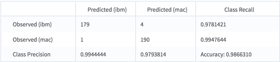
It predicts the correct class 98% of the time.