Example 5: Regression in Pieces
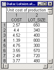
The logical operators demonstrated in the previous example can also be used in order to specify different regression models for different regions of the independent variable(s), that is, to estimate piecewise regression models (see the Introductory Overviews). This example is also based on a data set reported in Neter, Wasserman, and Kutner (1985, page 348). Specifically, the data set pertains to a production process in which the per-unit cost is related to the lot size and is shown in the Lotsize.sta data file. Open this data file by selecting Open Examples from the File menu (classic toolbar) or by selecting Open Examples from the Open menu on the Home tab (ribbon bar); it is in the Datasets folder.
Supposedly, for lots greater than 500, the relationship between the variables changes; Neter et al. (1985) fit a linear model that allows for different slopes for lots of sizes less than or equal to 500, and lots greater than 500. Specifically, Neter, et al. fit the following model:
y = b0 + b1*x + b2*(x-500)*(x>500)
Again, this model has a logical expression (x>500) that serves as a multiplier: If the expression is true, it will evaluate to 1; if it is false, it will evaluate to 0. Therefore, this equation actually represents two models. For values of x that are less than or equal to 500 (x>500 is false, i.e., equal to 0):
y = b0 + b1*x
For values of x that are greater than 500 [i.e., when (x>500) is equal to 1], the equation is:
y = b0 + b1*x + b2*(x-500)
If you multiply out this equation, you can see that for x values greater than 500, the slope is equal to b1+b2, and the intercept is equal to (b0-500*b2).
- Specifying the model
- As in
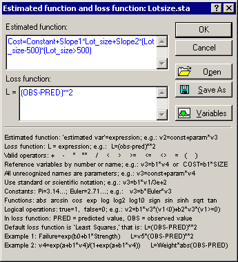
Example 4, specify the Estimated function (Cost=Constant+Slope1*Lot_size+Slope2*(Lot_size-500)*(Lot_size>500)) in the
Estimated function and loss function dialog.
As you can see, essentially you type in the equation in a straightforward manner. Note that in the illustration above, the variable names were used to denote variables, and the names Constant, Slope1, and Slope2 were used to denote the parameters. Remember that all unknown names will be interpreted by STATISTICA as model parameters. Also recall that you can record such long formulas via the Save As button in this dialog. They can later be opened via the Open button. You could also have used the Vxxx convention to refer to variables (where xxx is the variable number) and named the parameters a, b, and c. This would have saved you some typing but makes the formula less readable.
- Estimating the model
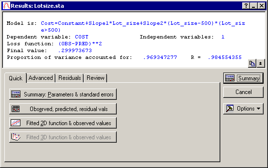
- Now, proceed as before, that is, accept all defaults in the Model Estimation dialog and click the OK button to display the Results dialog.
- Reviewing results
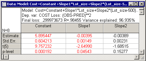
- Click the Summary: Parameters & standard errors button on the
Quick tab to display the parameter estimates in a spreadsheet.
The significance level for parameter Slope1 is .045; however, the other parameter is much less significant (.153), which may suggest that the initial (a priori) breakpoint (500) was adequate (i.e., the best regression models for the two ranges of Lot_size are different). In the next step, this will be more directly verified by estimating the value of the breakpoint itself.
- Estimating the breakpoint itself
- Logical expressions, such as the one used in this model, can also contain parameters (rather than constants only). For example, if you did not know where the breakpoint is in your model, you could specify the model as Cost=Constant+Slope1*Lot_size+Slope2*(Lot_size-Breakpnt)*(Lot_size>Breakpnt). (Click the Cancel button on the
Results dialog to return to the User-Specified Regression, Custom Loss dialog; then click the Function to be estimated & lost function button.)
Here, the parameter Breakpnt was added to the model. Thus, in this manner you can estimate the breakpoint. Continue to click the OK button until the Model Estimation dialog is displayed.
To estimate the above model, it is a good idea to set the start value for the Breakpnt parameter to about 500 (click the Start values button on the Model Estimation - Advanced tab). If you start the estimation with the default start values (0.1), then the Quasi-Newton estimation will move the breakpoint to negative values. Since there are no negative values in the data file, this is essentially like fitting a straight line without a breakpoint.
After you have specified the start values, click the OK button on the Model Estimation dialog to compute the estimates of parameters as well as of the Breakpnt; the Results dialog is then displayed. Now click the Summary: Parameters & standard errors button on the Results - Quick tab to produce the results spreadsheet containing the resulting parameter estimates (including the breakpoint) for this model and the related statistics.
Why not the Option "piecewise linear regression"? You may wonder why the piecewise linear regression model that is available on the Nonlinear Estimation Startup Panel was not used. That model allows you to specify or estimate breakpoints for the range of the dependent or y variable. Thus, that model was not applicable to this case.


