Example 5: Tweedie Distribution with Log Link
The data set used for this example is CarInsurance.sta, which contains damage claims for cars. Open the data set:
Ribbon bar. Select the Home tab. In the File group, click the Open arrow and from the menu, select Open Examples. The Open a STATISTICA Data File dialog box is displayed. CarInsurance.sta is located in the Datasets folder.
Classic menus. From the File menu, select Open Examples to display the Open a STATISTICA Data File dialog box; CarInsurance.sta is located in the Datasets folder.
- Specification of Distribution and Link Function
- Start the Generalized Linear/Nonlinear Models module:
Ribbon bar. Select the Statistics tab. In the Advanced/Multivariate group, click Advanced Models and select Generalized Linear/Nonlinear from the resulting menu.
Classic menus. From the Statistics - Advanced Linear/Nonlinear Models submenu, select Generalized Linear/Nonlinear Models.
The Generalized Linear/Nonlinear Models Startup Panel is displayed.
Select the Advanced tab. In the Distribution box, select Tweedie, and in the Link functions box, select Log.
In this Startup Panel, you can specify the index parameter (option Index Param) for the Tweedie distribution. This parameter must be between 1 and 2 and is used in specifying the variance function, V(µ) = µIndex parameter of the Tweedie distribution. For this example, specify 1.15 as the index parameter.
- Specification of Design
- Click the
OK button in the Generalized Linear/Nonlinear Models Startup Panel to display the
GLZ General custom design dialog box.
Click the Variables button to display the variable selection dialog box. Select ClaimAmount as the Dependent variable and HolderAge, CarGroup, and VehicleAge as the Categ. (factors), and then click the OK button.
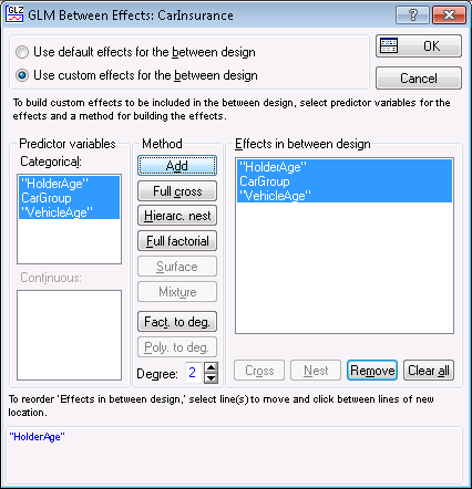
We want to specify only main effects in this design, so on the Quick tab, click the Between effects button to display the GLM Between Effects dialog box. Select the Use custom effects for the between design option button. Select all of the variables in the Categorical group box, and click the Add button.
Click OK in this dialog box, and click OK in the GLZ General custom design dialog box to display the GLZ -- Results dialog box.
- Parameter Estimates
- On the GLZ Results dialog box - Summary tab, click the Estimates button to review the parameter estimates for the model.
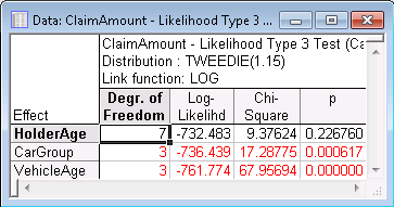
- Type 3 LR Test
- To determine significance of effects, click the Type 3 LR test button. This provides a test of the increment in the log-likelihood, attributable to the respective (current) effect, while controlling for all other effects. With a p-value < 0.01, VehicleAge and CarGroup are significant effects.
- Goodness of Fit
- The next step is to see whether, overall, this model provides a good fit to the data. Click the Goodness of fit button, located in the Sample group box, to display the Statistics of goodness of fit spreadsheet. If you compare the Scaled Deviance with its asymptotic chi-square with 114 degrees of freedom, the p-value is 0.88. This indicates a good model fit.
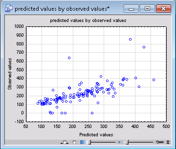
- Observed vs. Predicted.
- Now, select the Resid. 1 tab, and in the Plots of predicted and residual values group box, click the Observ. & pred. button to view how well the model fits the data. The graph indicates that the model fits the data reasonably well; however, it also indicates the presence of three outliers with extremely large observed values.