GLZ Results - Resid. 1 Tab
Select the Resid. 1 tab in the GLZ Results dialog box to access options to produce spreadsheets and plots of various basic predicted and residual statistics. For details regarding the computation and interpretation of these residual statistics, refer to McCullagh and Nelder, 1989.
Sample.
| Element Name | Description |
|---|---|
| Analysis, Cross-validation, Both | Select the respective option button under Sample to specify which type of sample to base the predicted and residual statistics. You can display spreadsheets for all observations that were used to compute the current results (select Analysis), all observations that were not used to compute the current results, but have valid data for all predictor and dependent variables (select Cross-validation), or all observations in both the Analysis sample and the Cross-validation sample (select Both). If these options are not available, no cross-validation sample was specified on the Quick Specs Dialog - Advanced tab, or via the Sample keyword in the Analysis Syntax Editor. |
| Basic Residuals | Click the Basic Residuals button to display a spreadsheet with the raw residuals, Pearson residuals, and deviance residuals; scaled Pearson residuals and scaled deviance residuals are also computed for continuous distributions (of the dependent (response) variable). |
| Predicted values | Click the Predicted values button to display a spreadsheet with the observed and predicted values, linear predictor values, their standard errors, and the confidence intervals for the predicted values. Cases with observed values that are outside the respective confidence interval for the predicted values will be highlighted in the spreadsheet.
As described in the Computational Approach section of the GLZ Introductory Overview, the relationship between predictors X1,..., Xk and (observed) response variable Y in the generalized linear model is assumed to be: Y = g(b0 + b1X1 + b2X2 + ... + bkXk) + e where b0, b1,..., bk are parameter estimates, e is the error, and g(...) is a known function. The items displayed in the spreadsheet can then be described as follows: Response value: The values of the response variable Y for each observation. Pred. value: Predicted values; the values of g(b0 + b1X1 + ... + bkXk) for each observation. Linear pred: Linear predictors; the values of b0 + b1X1 + ... + bkXk for each observation. Standard error: The estimates of the standard errors for the linear predictors for each observation. Lower CL: Lower confidence limits for the predicted values, for each observation. Upper CL: Upper confidence limits for the predicted values, for each observation. |
| Std. Residuals | Click the Std. Residuals button to display a spreadsheet with leverage values, studentized Pearson residuals, studentized deviance statistics, and likelihood residuals. |
| Class & odds ratio | This option is only applicable (available) for classification-type analyses (with a categorical dependent variable). Click the Classification of cases & odds ratio button to display a spreadsheet containing the classification of cases and odds ratios. |
| Other obs. Stats | Click the Other obs. Stats button to display a spreadsheet with generalized Cook's distances, differential chi-square values (measures the difference in the Pearson chi-square statistic due to removing the ith observation), and differential deviance residuals (measures the difference in the deviance statistic due to removing the ith observation). |
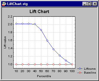
| Lift chart | This option is only applicable (available) for classification-type analyses (with a categorical dependent variable), when the categorical dependent variable is binary in nature, i.e., only contains two discrete values. The lift chart provides a visual summary of the usefulness of the information provided by a statistical model for predicting a binomial (categorical) outcome variable (dependent variable). Specifically, the chart summarizes the gain that you can expect by using the respective predictive model compared to using baseline information only.
For details regarding the interpretation of lift charts, see the Glossary entry by the same name. Refer also to the Rapid Deployment of Models module documentation for methods to produce overlaid (comparative) lift and gains charts for multiple predictive models and multinomial responses (with more than two categories). |
| Conf. lev | Enter the value to be used for constructing confidence limits in the respective results spreadsheets or graphs; by default 95% confidence limits will be constructed. |
| ROC curve | Click the ROC curve button to display the Goodness of Fit - ROC spreadsheet and ROC Curve graph. |
| Plots of predicted and residual values | The options under Plots of predicted and residual values are used to produce various plots of predicted and residual values. |
| Pred. values | Click the Pred. values button to produce a histogram of the predicted values. |
| Residuals | Click the Residuals button to produce a histogram of the raw residuals. |
| Observ. values. | Click the Observ. values button to produce a histogram of the observed dependent (response) variable values. |
| Pearson Resid | Click the Pearson Resid. button to produce a histogram of the Pearson residuals. |
| P-plot of observ | Click the P-plot of observ. button to produce a normal probability plot of the observed dependent (response) variable values; this option is only available for continuous distributions of the dependent (response) variable. |
| Pred. & resids | Click the Pred. & resids button to produce a scatterplot of the predicted values vs. the residuals. |
| Observ. & pred. | Click the Observ. & pred. button to produce a scatterplot of the observed values vs. predicted values. |
| Observ. & resids. | Click the Observ. & resids button to produce a scatterplot of the observed values vs. residuals. |
| Res. & case no | Click the Res. & case no. button to produce a scatterplot of the residuals vs. case numbers. |
| P-plot of resids | Click the P-plot of resids button to produce a normal probability plot of the raw residuals. |
| Bin number | Specify the number of bins you want to have on your histogram plots. This option applies to the histogram plots available on this tab (see above). Note that STATISTICA will not always produce histograms with the exact number of bins that you specify. It will produce the closest number to the specified bins while still maintaining "neat" intervals. |
| Aggregation | Select the Aggregation check box to compute the predicted values (and related statistics, e.g., residuals) in terms of predicted frequencies. In models with categorical response variables, predicted values (and related statistics, e.g., residuals) can be computed in terms of the raw data or for aggregated frequency counts. For example, in the Binomial case (see
Distribution and link function), and for raw data, you can think of the response variable as having two possible values: 0 (zero) or 1. Accordingly, predicted values should be computed that fall in the range from 0 (zero) to 1 (e.g., classification probabilities). If the Aggregation check box is set (also available on the
Summary tab), then STATISTICA will consider the aggregated (tabulated) data set. In that case, you can think of the response variable as a frequency count, reflecting the number of observations that fall into the respective categories. This is easiest imagined in the case where the predictors are also categorical in nature: The resulting aggregated data file would simply be a multi-way frequency table.
See the Results for stepwise or best-subset regression and Overdispersion parameter for models with categorical responses notes in GLZ Results for further information. See also, GLZ - Index. |