Example 4: Stub-and-Banner Tables

Overview. Stub-and-banner tables are an economical way to report several two-way tables simultaneously. To continue the analysis of Example 3: Frequency Tables, it is desired to learn whether the same respondents in the survey who expressed the greatest interest in football also expressed the greatest interest in baseball and basketball. As mentioned earlier, if this is the case, then perhaps it would be sufficient to show one of those sports on one TV screen, and show something entirely different on the other; this way you can attract a new and different clientele. To examine the overlap between sports, that is, the extent to which respondents' interest in football is correlated with that in other sports, compute a stub-and-banner table.

Specifying the Analysis. Open the Sports.sta data file. This data file is described in Example 3. Then, start the Basic Statistics and Tables module.

Ribbon bar. Select the Home tab. In the File group, click the Open arrow and on the menu, select Open Examples. The Open a Statistica Data File dialog box is displayed. Sports.sta is located in the Datasets folder. Then, select the Statistics tab. In the Base group, click Basic Statistics to display the Basic Statistics and Tables dialog box.

Classic menus. From the File menu, select Open Examples to display the Open a Statistica Data File dialog box; Sports.sta is located in the Datasets folder. Next, from the Statistics menu, select Basic Statistics/Tables to display the Basic Statistics and Tables dialog box.

Double-click Tables and banners to display the Crosstabulation Tables dialog box. Select the Stub-and-banner tab.

Layout of the table. The stub-and-banner table basically consists of a number of two-way tables put together. The best way to illustrate how these tables are constructed is to review a typical stub-and-banner table. Therefore, in the Crosstabulation Tables dialog box, click the Specify tables (select variables) button to display the variable selection dialog box.

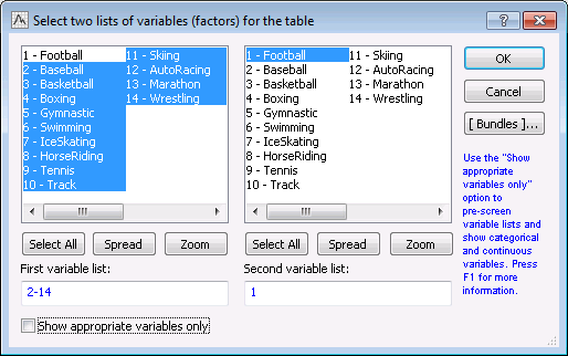
For this example, select variables 2-Baseball through 14-Wrestling as the row variables from the First variable list and variable 1-Football as the column variable in the Second variable list.

Click the OK button to finalize the selection, and then click the OK button in the Crosstabulation Tables dialog box to display the Crosstabulation Tables Results dialog box. On the Quick tab, click the Stub-and-banner table button to produce the spreadsheet of results.

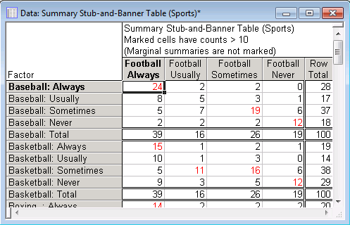
Reading the Table. Again, you can think of this table as a combination of different two-way tables. For example, the first four rows of the table show the frequencies in the two-way tables of Football by Baseball. Put another way, you can see the (joint) distribution of the 100 respondents across the 4*4=16 cells created by the crosstabulation of respondents' interest in watching football by their interest in watching baseball. Now try different ways of expressing the results.

Raw frequencies. By default, the stub-and-banner table will contain raw frequencies, as shown above. Thus, you can see that 24 (out of the 100 respondents) reported being always interested in watching football and always interested in watching baseball. Looking at the first three rows of the right-most column, you can see that of those respondents who say they are never interested in watching football, only 7 (0+1+6) report being interested in baseball Always (0), Usually (1), or Sometimes (2). Therefore, it looks like the two sports, football and baseball, to a large extent appeal to the same people.

Percentages. Now, return to the Crosstabulation Tables Results dialog box, which contains options that enable you to express the entries in the table in terms of column percentages, row percentages, or total percentages. You can also elect to include expected and/or residual frequencies in the stub-and-banner table.

Select the Options tab. In the Compute tables group box, select the Percentages of row counts check box.

Select the Quick tab, and click the Stub-and-banner table button.

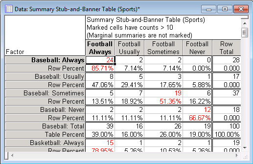
When you select the Percentages of row counts check box, the Display selected %'s in sep. tables check box becomes available on the Advanced tab. Because so much information can be included in one table, selecting this check box will place the row percentages in a separate spreadsheet from the raw frequencies.

Look at the first row in the spreadsheet shown in the above image. You can see that of those respondents who said they are Always interested in baseball (all respondents in the first row), 85.71% say they are Always interested in football as well.

Finding a sport unrelated to football. Look at the total percentages in order to find a sport that is not related to football. Return to the Crosstabulation Tables Results dialog box and select the Options tab. In the Compute tables group box, select the Percentages of total count check box (for simplicity, clear the Percentages of row counts check box).

Click the Stub-and-banner table button on the Quick tab to produce the spreadsheet with these counts.

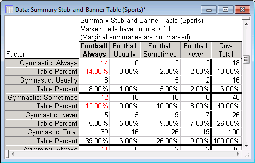
Scroll the spreadsheet down until you can view the counts for Gymnastic (see above). The entries in this table are now total percentages. Thus 14 percent of all respondents report to be Always interested in Football and Always interested in Gymnastics. Only 7 percent of the respondents say that they are Never interested in Football and Never interested in Gymnastics. At the same time, 12 percent (2+2+8) of the respondents say that they are Never interested in Football, but either Always (2%), Usually (2%), or Sometimes (8%) interested in Gymnastics. Thus, gymnastics would seem to be a nice programming alternative (for the second large-screen TV in your bars) to football, baseball, or basketball, and may attract at least some different customers.

Statistics. The Introductory Overview reviews some of the statistics commonly used to express contingency or relationships between two categorical variables. Let's look at some of those statistics, which are listed in the Crosstabulation Tables Results dialog box, on the Options tab in the Statistics for two-way tables group box. The most commonly used statistic of contingency between two categorical variables is the Chi-square test; therefore, select the Pearson & M-L Chi-square check box.

A measure of correlation similar to the Pearson r is the Spearman R, or Rs. This measure assumes that the values for the variables contain at least rank order information. This assumption is reasonable in this example since a person who reports to be Always interested in watching football is probably more of a football fan than a person who reports being only Usually interested. Therefore, also select the Spearman rank order correlation check box.

Selecting a table. Now that the statistics selections have been made, select the Advanced tab, and click the Detailed two-way tables buttons. The Select the tables you want to review dialog box is displayed, in which all available two-way tables will be listed.

You can select the desired tables from this list, or select All Tables to produce all two-way tables. For this example, select the Baseball Football table and click the OK button. Two spreadsheets are produced for each table selected.

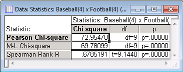
The first spreadsheet (2-Way Summary Table) contains the observed (raw) frequencies and any other selections made in the Compute tables group box of the Crosstabulation Tables Results dialog box - Options tab (e.g., Percentages of total count). The second spreadsheet (Statistics) contains the Chi-square tests and Spearman correlation results.

The Pearson Chi-square value for this two-way table is 72.95, which is statistically significant (refer to Elementary Concepts, for an explanation of significance testing). The Spearman Rank R is equal to 0.6785, reflecting the substantial correlation between interest in football and baseball in this sample.

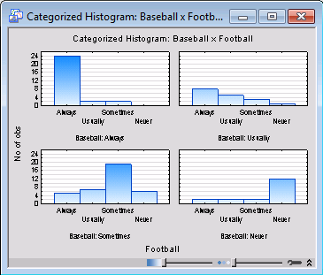
Click the Categorized histograms button on the Advanced tab of the Crosstabulation Tables Results dialog box (select the Baseball Football table in the Select the tables you want to review dialog box),

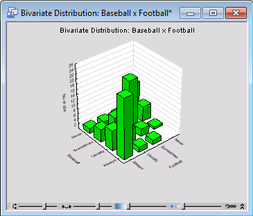
or the 3D histograms button,

to visually inspect the frequencies of the selected two-way tables. Note that you can use the Interactive Graphics Controls at the bottom of the graph window to rotate the graph and/or adjust the transparency of the plot areas to view different aspects of the plot.

Reviewing other tables. Return to the Crosstabulation Tables Results dialog box, and on the Advanced tab click the Detailed two-way tables button.

Select the table Gymnastic Football in the Select the tables you want to review dialog box and click the OK button. (The same statistics will be computed for this table since you did not make any new selections among those options.)

There is still a relationship between reported interest for Football and Gymnastics. However, it is not nearly as strong (the Spearman Rank R is computed as 0.33). The fact that even this variable (Gymnastic) is significantly related to football suggests that many of the respondents (sampled from within the sports bars) are indeed generally interested in watching all kinds of sports.

Summary. The major results of this analysis are that 1) most of the respondents in the survey were interested in watching all major sports, that is, football, baseball, and basketball, and 2) showing gymnastics from time to time may appeal to at least some respondents who explicitly are not interested in watching football.

See also, the Basic Statistics and Tables Index and Overviews.