Distributions & Simulation Example

Overview

The Distributions & Simulation module is used to evaluate the fit of theoretical distributions to observed data. In addition, you can simulate data from those theoretical distributions with the choice of incorporating the correlation structure of the data. Although seemingly simple, this module enables you to accurately model the current processes that generate the data, and from there you can simulate from those processes, and evaluate the performance of a system.  

For this example, assume that we are manufacturing a hinge that has four parts.

If the sum of the first three parts is greater than the width of the last part, then the product is defective.

Instead of having to wait to accrue the required data, you can

1. fit theoretical distributions to the observed data
2. simulate from those distributions
3. draw conclusions based upon the simulation (for example, determining the percentage of defectives, etc.)

Specifying the Analysis

1	Open the SimulationRiskData.sta data file.
2	Start the Distributions & Simulation module.
3	Select the Home tab.
4	In the File group, click the Open arrow.
5	Select Open Examples	The Open a Statistica Data File dialog box displays. The SimulationRiskData.sta data file is located in the Datasets folder.
6	Select the Statistics tab.	The Statistics options display.
7	In the Base group, click More Distributions.	The Distributions & Simulation Startup Panel displays.
8	On the Quick tab, select Fit Distribution.	The Distributions & Simulation dialog box displays.
9	Click the OK button.	The Fit Distributions dialog box displays.

Select Variables

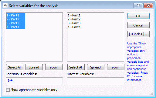
1	On the Quick tab, click the Variables button.	The Variable selection dialog box displays.
2	Select variables 1-4 as the Continuous variables.
3	Click OK.	The variable selection dialog box closes.
4	In the Fit Distributions dialog box, select the Continuous variables tab	The available distributions to fit to the observed data display.
5	On this tab, select which distributions you want to fit to the observed data. For this example,fit all distributions to each variable (already selected by default).
6	Click the OK button.	The analysis will run., and once they are complete, the Fit Distributions Results dialog box will display.

View the Results

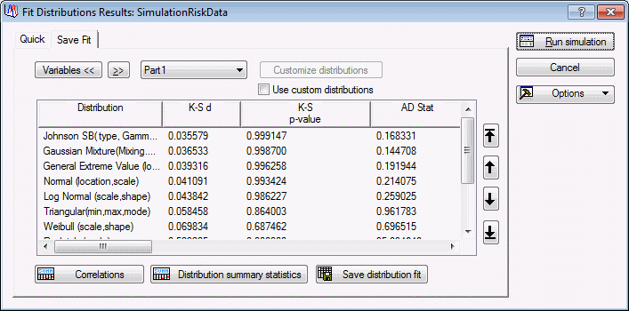
1	Select the Save Fit tab.	The results will display, showing which distribution was considered the best fit for each selected variable. By default, Part1 is selected. According to the p value of the K-S test, the Johnson SB distribution is the best fit for Part1.
2	Click the >> button to scroll through the distributional fit results of Part2, Part3 and Part4.	According to the K-S test, the Gaussian Mixture is the best fit for Part2 and Part3, and the Johnson SB distribution is the best for Part4.
3	Select the Quick tab.	The options to create graphs to help you visualize the results of the analysis will display.
4	Select Part1 if it is not already selected by default in the Variables drop-down list.
5	From the Distribution drop-down list, select Johnson.
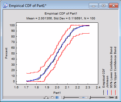
6	Click the Empirical CDF plot button.	The Empirical Cumulative Distribution Function plot displays
7	Click the Q-Q plot button.	The Quantile-Quantile plot displays.
8	Use the Interactive Graphics Controls at the bottom of the graph window to adjust the transparency of the markers.	Both of these plots show that the Johnson distribution is a good fit to the observed data for Part1.
9	Do the same for the remaining variables.

Run a Simulation

For this example, continue with the analysis.

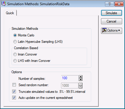
1	Click the Run simulation button.	the Simulation Methods dialog box displays. Since the four parts are not independent of one another, you need to incorporate the correlation structure.
2	Select Iman Conover as the simulation method.
3	Set the Number of Samples to 100,000.
4	Click the Simulate button.	The results spreadsheet will display.
5	Select the Data tab (in Statistica).
6	In the Mode group, select the Input check box.

Create a New Variable

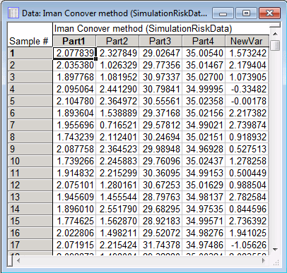
Since a defect is defined as an item where the sum of the first three parts is greater than the fourth part, create a new variable that describes this relationship of defects to the four parts. Use the following spreadsheet formula: v4-v1-v2-v3.

1	Right-click on any of the variable headers in the spreadsheet, and from the shortcut menu select Add Variables.	The Add Variables dialog box displays.
2	Double-click in the After edit box.
3	Select Part4, and click OK.
4	In the Add Variables dialog box, in the Long name (label or formula with Functions) edit box, enter the formula =v4-v1-v2-v3.
5	Leave all other defaults, and click OK.	A new variable called NewVar is created in the spreadsheet.

Create a Histogram

To view the distribution of the new variable, we will create a histogram of the data.

	Select the Graphs tab. in the Common group, and click Histogram.	The 2D Histograms Startup Panel displays.
	Click the Variables button, and select NewVar.
	Click the OK button.
	Click OK in the 2D Histograms Startup Panel.	You will see that a small percentage ( fewer than 0) of cases are defective. A defect is defined as the sum of the first 3 parts being greater than the forth, v1+v2+v3>v4. With some simple math, this is rewritten as: v4-v1-v2-v3<0. The percentage of defectives from the simulated data is about 10%. Further results might be gleaned from the simulated data, such as computation of certain quality or process-related statistics such as cpk, etc. The simulated results can then be used to guide engineers to change certain aspects of the production process.