Example 7: Taguchi Robust Design Experiment
This example is based on data presented by Phadke (1989) on the manufacture of polysilicon wafers. It is assumed that you have read the section on Taguchi methods in the Introductory Overview. The purpose of the study was to reduce:
The control factors in this study were:
Each factor was set at three levels.
Open the Taguchi.sta data file.
Ribbon bar. Select the Home tab. In the File group, click the Open arrow and from the menu, select Open Examples to display the Open a Statistica Data File dialog box. Double-click the Datasets folder, and open the Taguchi.sta data set.
Classic menus. On the File menu, select Open Examples to display the Open a Statistica Data File dialog box. The Taguchi.sta data file is located in the Datasets folder.
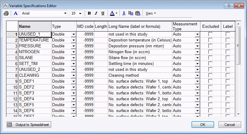
Details concerning the specific settings for each variable in the data file can be viewed in the Variable Specifications Editor.
Ribbon bar. Select the Data tab. In the Variables group, click All Specs.
Classic menus. On the Data menu, select All Variable Specs.
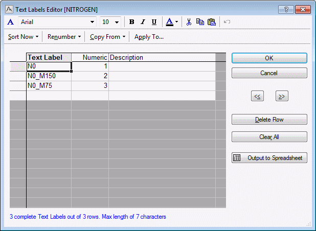
Also, see the Text Labels Editor. First, in the spreadsheet, select the variable of interest.
Ribbon bar. Select the Data tab. In the Variables group, click Text Labels.
Classic menus. On the Data menu, select Text labels Editor.
The text labels shown below are for variable 4.
For this example, a Taguchi design will first be generated.
- Generating the Design
- Start the Experimental Design (DOE) analysis:
Ribbon bar. Select the Statistics tab, and in the Industrial Statistics group, click DOE to display the Design & Analysis of Experiments Startup Panel.
Classic menus. On the Statistics - Industrial Statistics & Six Sigma submenu, select Experimental Design (DOE) to display the Design & Analysis of Experiments Startup Panel.
Select the Advanced tab, select Taguchi robust design experiments (orthogonal arrays), and click OK.
In the Design & Analysis of Taguchi Robust Design Experiments dialog box, select the Design experiment tab.
For this example, select array L18.
This array will suit the study very well. In 18 runs, it will accommodate up to 8 factors total and up to 7 three-level factors. In this study, there are 5 three-level factors, so some of the columns of this array will simply be unused.
The name orthogonal arrays denotes the fact that the columns of the array are independent of each other. If you simply ignore some columns, but complete all 18 runs, the remaining columns are still orthogonal to each other, and the effects of the control factors can be estimated.
- If your design does not fit any of those listed
- Taguchi (1987, Chapter 38) discussed in detail how the orthogonal arrays are constructed. More importantly, in some instances, ignoring columns allows you to estimate unconfounded interactions. Also, in some instances you can combine columns (factors) to form new orthogonal factors with more levels.
A technical discussion of these techniques is beyond the scope of the example; however, if your particular design does not fit any of those listed here, you can refer to Taguchi (1987) or Phadke (1989) for methods of "customizing arrays" (specifically, refer to the use of linear graphs in those sources to learn how to manipulate the columns of orthogonal arrays).
- Reviewing the design
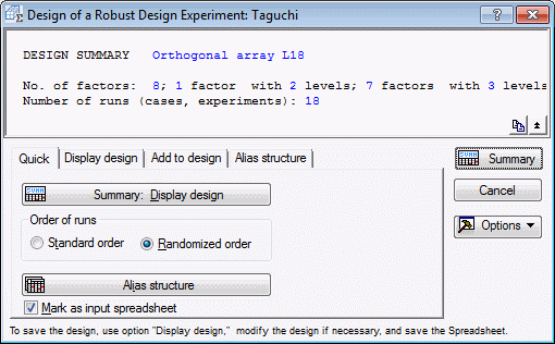
- In the Design & Analysis of Taguchi Robust Design Experiments dialog box, click OK to display the Design of a Robust Design Experiment dialog box
In the Order of runs group box, select the Standard order option button, and click the Summary: Display design button to produce the design in a spreadsheet.
As before, you can randomize the runs in the spreadsheet and add blank columns to produce convenient data entry forms.
- Alias structure
- Now, click the Alias structure button to review the matrix of aliases of two-way interactions. A message will be displayed. Click OK.
Each asterisk in this spreadsheet shows how a particular interaction (column) is confounded (completely or partially) with a respective main effect (row). Apparently, the factor 1 by factor 2 interaction (first column) is not confounded with any main effects. Thus, if you had a two-level factor in this example study (which is not the case; see above), you could, using array L18, estimate the two-way interaction between the first two factors.
- Analyzing the design
- As mentioned earlier, the data file Taguchi.sta contains the results of this study. This file contains detailed text values and variable labels, and you may want to review them at this point. However, the nature of the variables will be described as they are encountered in the example.
- Specifying the design
- In the Design of a Robust Design Experiment dialog box, click the Cancel button to display the
Design & Analysis of Taguchi Robust Design Experiments dialog box. Select the
Analyze design tab.
First, analyze the surface defect data. Ideally, you want to have no surface defects at all on the wafers, so this constitutes a smaller-the-better type of problem. The different signal to noise (S/N) ratios are in the Introductory Overview.
In the Problem type drop-down list, select Smaller-the-better .
All that is left now is to specify the variables. Click the Variables button, and in the variable selection dialog box, select as the Dependent variables the 9 measures of the number of surface defects, that is, select variables S_def1 to S_def9.
The Independent vars (factors) are variables Temperature through Sett_tim and variable Cleaning. Remember that orthogonal array L18 can accommodate up to 8 factors, of which only 6 need to be used; thus, variables 1 and 7 will not be used.
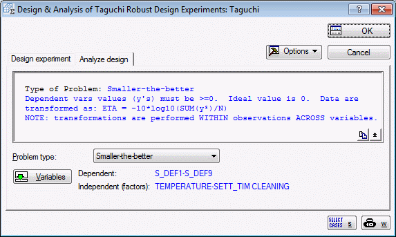
Click OK, and the Design & Analysis of Taguchi Robust Design Experiments dialog box will now look like this:
- Reviewing results
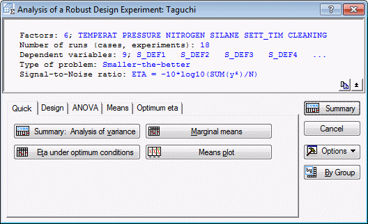
- Now, click OK to execute the analysis and display the Analysis of a Robust Design Experiment dialog box, which contains numerous options available to review the raw data as well as the S/N ratios for each run.
- Reviewing marginal means
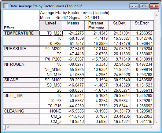
- Click the Marginal means button to review a spreadsheet of the marginal means.
This spreadsheet shows the means (for Eta, the S/N ratio) for each level for each factor; also computed (in the third column) are the parameter estimates, that is, the deviations of the mean of the respective factor level from the overall mean (μ). Remember that you want to maximize the S/N ratios, so for example, for factor Temperature, the largest S/N ratio occurred in level 1 (T0_M25).
You can plot all of these means in a summary plot by clicking the Means plot button. However, before you look at this plot, look at the ANOVA spreadsheet, because the standard errors reported in the plot depend on your selections in this spreadsheet.
- Reviewing the ANOVA table
- Return to the Analysis of a Robust Design Experiment dialog box, and click the Summary: Analysis of variance button, which can be found on the
Quick tab or the
ANOVA tab.
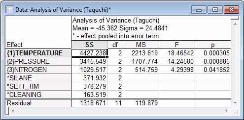
Customarily, to obtain a more stable estimate of the error variance, small and nonsignificant effects are pooled into the error term. Even though this procedure capitalizes on chance (and the resultant p values are suspect), it yields more stable predictions later (see below).
To pool an effect into the error term, select the ANOVA tab. Select the Pool some effects check box, which will cause the Select effects to be pooled dialog box to be displayed. For this example, select the Cleaning effect and click OK to pool it into the error term. Then, click the Summary: Analysis of variance button again.
Note: you can "unpool" effects (that is, place them back into the estimate) by clearing the Pool some effects check box. For now, however, leave Cleaning in the error term and, in addition, pool factors Silane and Sett_tim into the error term: click the Select button next to the Pool some effects check box, select these additional factors, and click OK.Click the Summary: Analysis of variance button again.
- Plot of means
- Return to the Analysis of a Robust Design Experiment dialog box, and click the Means plot button (either on the
Quick tab or the
Means tab).
Note: the dashed lines in the above plot indicate the 2 times standard error limits around the mean Eta. This standard error is computed from the last error term that you specified in the previous spreadsheet, that is, with three effects pooled into the error. The regular error term (without any interactions) from the overall analysis is used if no specific pooling was previously selected. In this plot you can easily identify the best settings for each factor, that is, the ones that maximize the S/N ratio. Note that although factor Nitrogen was significant, none of the settings resulted in effects greater than the 2 times standard error limits of Eta; thus, the utility of this factor is also suspect. Now, return to the Analysis of a Robust Design Experiment dialog box.
Predicting Eta, verification experiments. As previously mentioned, pooling non-significant effects into the error term capitalizes on chance, and you may find seemingly significant factors by pure chance.
One way to "verify" your results is by first predicting Eta under optimum conditions, based on the factors that you have identified as being significant, that is, Temperature and Pressure in this case. Then you could run a verification experiment, that is, a few number of runs using those actual settings. If sizable differences between predicted and observed values occur, you have either erroneously included factors that were not significant, or there are unexpected interactions among the factors. Both cases are discussed in detail in Phadke (1989).
In summary, you should try (in that case) to rescale your measures or levels so that no significant interactions remain. You can use the traditional two-level factorial designs (of sufficient resolution) to detect interactions in your data.
Now, turn to the prediction of Eta. In the Analysis of a Robust Design Experiment dialog box, click the Eta under optimum conditions button (either on the Quick tab or the Optimum eta tab).
Note that, on the Optimum eta tab, you can again choose whether to pool some effects into the error term. You can also include previously excluded factors with this option.
The other options available pertain to the actual settings for each factor. By default, all levels will be set to their optimum, that is, to the levels that produce the largest S/N ratio. You can change those settings by selecting the Set selected factors at specific levels check box, and then the User-Defined Factor Settings dialog box will be displayed, in which you can select the desired levels for the respective factor.
For now, leave these settings at their defaults.
- Accumulation analysis
- Before concluding this example, look at the data on the cumulative number of surface defects found in the sample. In the data file Taguchi.sta, variables D_0_3 to D_1001__ contain the number of defective surfaces found in each run, categorized into intervals.
Overall, in each run, 9 surface samples were inspected. The frequencies in variable D_0_3 represent the number of surfaces found with 0 to 3 defects, variable D_4_30 contains the number of surfaces found with 4 to 30 defects, and so on. Such categorical frequency data can be analyzed via accumulation analysis.
Return to the Design & Analysis of Taguchi Robust Design Experiments dialog box by clicking the Cancel button in the Analysis of a Robust Design Experiment dialog box.
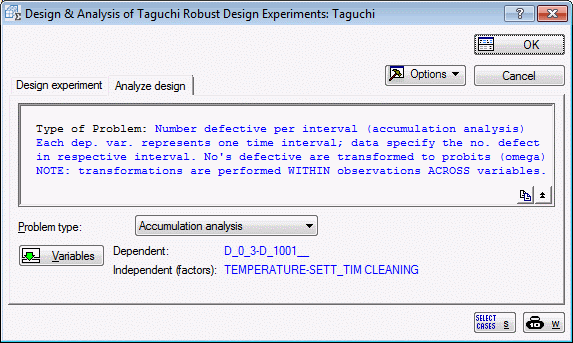
Select Accumulation analysis in the Problem type drop-down list.
Next, click the Variables button and in the variable selection dialog box, select variables D_0_3 through D_1001__ as the Dependent variables, and select the same Independent vars (factors) as before (variables Temperature through Sett_tim, and variable Cleaning). Click OK.
- Results of accumulation analysis
- Now, click OK to view the results of this analysis in the
Accumulation Analysis Results dialog box.
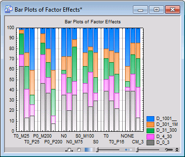
ANOVA results are not available for this type of analysis (because they are not appropriate). However, you can visualize the results via bar plots. Click the Bar plot of cumulative proportions button to produce the plot.
In this plot, the relative frequencies (proportions) in each category (D_0_3 through D_1001__) for each level of each factor are shown in stacked columns. For example, for the first factor (Temperature), we can immediately recognize that the largest area of shading occurs under level T0_M25.
This information for this factor can also be displayed via a line plot of the cumulative proportions across categories. Click the Line graph by factor button, and in the Select factor for line plot dialog box, select the factor Temperature. Click OK.
As shown in the illustration above, the line indicating the cumulative proportion defective is highest for level T0_M25; thus, most surfaces under that setting for that factor had 3 or fewer (D_0_3) defects.
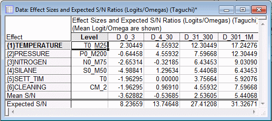
Predicting Eta under optimum conditions. The Eta under optimum conditions button works as before, except that predictions are made in terms of logits (see the Introductory Overview; Taguchi refers to these values as omega transformed frequencies) that are computed for each category.
Summary. To summarize the analyses, it appears that the factors Temperature and Pressure had the greatest effect on surface defects found on the polysilicon wafers. Setting both factors at their first levels (T0_M25 and P0_M200, respectively) yielded the best results, that is, lowest number of surface defects. You can now proceed to analyze the data for the surface thickness (variables Thick_1 through Thick_9). Note that those data represent a nominal-the-best problem; that is, a constant thickness of the polysilicon layer is desirable.
See also, Experimental Design Index.

