Multidimensional Scaling - Example

Overview and Data File

This example is based on the data file Nations.sta. These data are discussed in Kruskal and Wish (1978, page 30). The data file contains the mean similarity ratings of 18 students for 12 countries. The countries are Brazil, Congo, Cuba, Egypt, France, India, Israel, Japan, Mainland China, Russia, USA, and Yugoslavia. A partial listing of this similarity matrix is shown in the following image.

Note: You can produce a similar matrix file by entering the distances into a new spreadsheet following the matrix data format conventions (as described in the Matrix File Format topic).

This test case explains Multidimensional Scaling functionality in a number of steps.

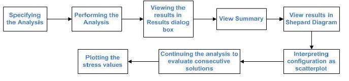
Specifying the Analysis

Open the Nations.sta data file, and start the Multidimensional Scaling module:

1. To display a standard Variable Selection dialog box, click the Variables button on the Quick tab in the Startup Panel.
2. Select all the variables for the analysis, and then click OK to close the Variable Selection dialog box and return to the Startup Panel.
   

   Statistica assumes that you want to calculate a two-dimensional solution for this similarity matrix, and that the initial solution is to be estimated via principal components analysis.

3. Alternatively, on the Options tab, you can also specify the initial configuration by selecting a Statistica raw data file with the initial coordinates.
4. To simply accept the default settings, click OK.
5. The initial configuration is computed first, and the Parameter Estimation dialog box is displayed.
   Note: You can later view these initial configurations by clicking the Start (initial) configuration button on the Results dialog box - Review & Save tab.

   Go back to the flow diagram.

Performing the Analysis

After specifying the analysis, you can perform the analysis.

1. The iterative algorithm for finding an optimum configuration proceeds in two stages:
   • First, Statistica uses a method known as steepest descent. The respective number of steepest descent iterations is listed in the Parameter Estimation dialog box in the first column labeled iter. s.
   • After each iteration under steepest descent, Statistica performs up to five additional iterations to regulate the configuration. For details, see Technical Notes. The respective numbers of these iterations are listed in the Parameter Estimation dialog box in the second column labeled iter. t.
2. In addition, the stress value and coefficient of alienation are calculated and displayed at each step. A detailed discussion of this iterative procedure can be found in Shiffman, Reynolds, and Young (1981, pages 366-370).
   
3. After Statistica has determined the best two-dimensional configuration, it displays the final stress value.
4. To display the Results dialog box, click OK.

Go back to the flow diagram.

Results

You can examine the results in spreadsheets or graphs using the options available in the Results dialog box.

First, examine the table of actual distances and estimated distances.

Go back to the flow diagram.

Reproduced and observed distances

To evaluate the fit of the two-dimensional solution, click the Summary statistics button on the Advanced tab.

The columns labeled D-hat and D-star contain the monotone transformations of the input data: D-stars are rank images calculated according to Guttman (1968); D-hats are monotone regression estimates calculated according to Kruskal (1964).

The rows in the spreadsheet, each representing one distance as specified in the similarity matrix, are sorted according to the size of D-star or D-hat. The second column of the spreadsheet contains the reproduced Distances from the current configuration. If the fit of the current model, that is the current number of dimensions, is very good, then the order of reproduced distances must be approximately the same as that for the transformed input data. Example, D-star or D-hat values. Out-of-order elements indicate lack of fit. The first column of the spreadsheet references the elements of the original input matrix as D(X,Y), where X is the respective row in the input matrix, and Y is the respective column.

For example, D(2,1) is the element in the second row and the first column of the input matrix. In our example, the comparison between Congo and Brazil. It appears that the order of distances was approximately reproduced by the two-dimensional solution.

Go back to the flow diagram.

Shepard diagram

Now examine the Shepard plot. This plot is a scatterplot of the observed input data (similarities or dissimilarities) against the reproduced distances. The plot also shows the D-hat values, that is, the monotonically transformed input data, as a step function. To produce this plot, click the Shepard diagram button on the Quick or Advanced tab.

Most points in this plot are clustered around the step-line. Thus, you might conclude for now that this two-dimensional configuration is adequate for describing the similarities between countries.

Go back to the flow diagram.

Interpreting the configuration

The actual orientation of axes in multidimensional scaling is arbitrary, just as in Factor Analysis. Thus, you can rotate the configuration to achieve a more interpretable solution.

Kruskal and Wish (1978) used a program called KYST (named after Kruskal, Young, Torgeson and Shepard) that used a slightly different algorithm for multidimensional scaling to analyze the present data, and they obtained a very similar solution. Then they rotated their solution by approximately 45 degrees, and interpreted the rotated dimensions as developed vs. underdeveloped, and pro-western vs. pro-communist. Looking at the following plot and mentally rotating it by 45 degrees, this interpretation seems to hold quite well. Remember that this study was conducted in the 1970's.

In this plot the scaling is adjusted using the Scaling tab in All Options dialog box. In addition to meaningful dimensions, you must also look for clusters of points or particular patterns and configurations such as circles, manifolds, etc. For a detailed discussion of the way to interpret final configurations, see Borg and Lingoes (1987), Borg and Shye (in press), or Guttman, (1968).

Go back to the flow diagram.

Continuing the Analysis

1. To return to the Multidimensional Scaling Startup Panel, click the Cancel button in the Results dialog box.
2. Select the Options tab.
   
   Note: Now the default settings on the Options tab are different than when the program was first started. Multidimensional Scaling remembers the configuration from the previous analysis, unless you specify a new data file or if you select new cases. Also, the default Number of dimensions on the Quick tab is now 1.
3. You can click OK to compute the one-dimensional solution, using the configuration for the first dimension from the previous analysis as the starting configuration. In this way, you can efficiently evaluate several consecutive solutions, starting with several dimensions and getting one-dimensional solution.

Go back to the flow diagram.

Scree test: Plotting the stress values

This example began with the two-dimensional solution. If you are unsure about the dimensionality underlying the matrix, you must plot the stress values for consecutive numbers of dimensions. Then, find the place where the smooth decrease of stress values appears to level off to the right of the plot. To the right of this point, presumably, one finds only factorial scree. Scree is the geological term referring to the debris that collects on the lower part of a rocky slope (see, for example, Kruskal and Wish, 1978, pages 53-56, for a discussion of this plot). The following scree plot was created by first creating a new spreadsheet containing the D-star: Raw stress values (that can be found in the Results dialog box summary box) for consecutive dimensions (1 through 6) for the present data,

and then selecting Line Plot (Variables) on the Graphs - 2D Graphs tab or menu.

Based on the preceding plot, the two-dimensional solution is chosen. You can also look at the three-dimensional solution. You can be the judge of whether the three-dimensional solution is more meaningful than the two-dimensional one.

Following is a 3D scatterplot of the solution when 3 is specified as the Number of dimensions on the Multidimensional Scaling Startup Panel - Quick tab. To produce this graph, click the Graph of final configuration, 3D button on the Results - Quick tab. This button is disabled if 1 or 2 dimensions were specified in the Startup Panel; note that when you click this button you are prompted to select the dimensions to plot in the 3D graph using the Select three dimensions for scatterplot dialog box.

Go back to the flow diagram.