Monte Carlo Example 2: Performance of GLS and ML Estimation in the Comparison of Correlation Matrices

In the example on comparison of correlation matrices (see Example 18: Testing the Equality of Correlation Matrices from Different Populations), we found that the Chi-square statistic based on the ML estimation procedure produced a rejection of the null hypothesis at the .05 significance level, while the analogous statistic based on GLS estimation failed to reach significance. This contrast raised questions about the relative performance of the two methods. It could be that the difference relates solely to the difference in power between ML and GLS methods. (ML methods are generally somewhat more powerful.) However, the ML procedure may be excessive (i.e., reject a true null hypothesis more frequently than the nominal rate) at the rather small sample sizes used in the Jennrich (1970) example (Jennrich himself questions the adequacy of the sample sizes in his original paper). Structural Equation Modeling provides tools for delving further into these questions. Specifically, you can perform a Monte Carlo study to assess the relative Type I error rates for the GLS and ML estimation procedures.

A full Monte Carlo study to examine the general question of relative performance of the GLS and ML statistics would, of course, require many conditions, varying relative sample sizes, and the characteristics of the population correlation matrices being simulated. This example demonstrates how to set up one highly relevant condition from such a study.

The simulation examined here assumes that the population correlation matrices are, in fact, the same, and that sample sizes are 90 and 40, roughly equivalent to those in the Jennrich example. This simulation is rather time-consuming. Typically, each replication will require approximately 3 minutes on a computer with a 486DX-33 processor. A set of 100 replications would, thus, require about 5 hours on a 486-33 (about 50 minutes on a 100 Mhz Pentium-based computer). Depending on your computer's microprocessor, you may have to schedule this example for a time (possibly overnight) when the computer will not be required for other purposes.

The Monte Carlo study requires two runs. The first run collects data for the Maximum Likelihood discrepancy function, the second run gathers data for the GLS discrepancy function.  

A problem is specifying reasonable choices for the hypothetical population correlation matrices for the Monte Carlo study. A choice that seems natural and eminently reasonable in this case is to use, as the hypothetical population, the estimates for the population parameters obtained when testing the hypothesis of equal correlation matrices with a particular estimation procedure. When treated as population values, these estimates will, of necessity, specify a situation where the null hypothesis is true.

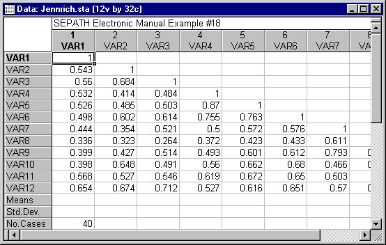
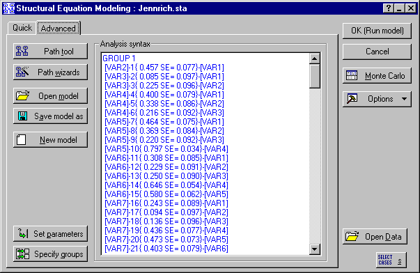
In Example 18 of the Structural Equation Modeling examples, we tested the hypothesis of equal correlation matrices using GLS estimation. The parameter estimates for that analysis have been incorporated into PATH1 statements to create the model in the file Monte2GL.cmd, which can be found in the examples directory. This file will serve as the population model for the Monte Carlo study.

Ribbon bar. Select the Home tab. In the File group, click the Open arrow and select Open Examples to display the Open a STATISTICA Data File dialog box. Open the Datasets folder. Open the data file, which is located in the SEPATH folder. Then, select the Statistics tab. In the Advanced/Multivariate group, click Advanced Models and from the menu, select Structural Equation to display the Structural Equation Model Startup Panel.

Classic menus. From the File menu, select Open Examples to display the Open a STATISTICA Data File dialog box. Open the Datasets folder. Open the data file, which is located in the SEPATH  folder. Then, from the Statistics - Advanced Linear/Nonlinear Models submenu, select Structural Equation Modeling to display the Structural Equation Model Startup Panel.

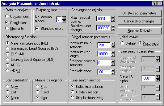
Click the Set parameters button to display the Analysis Parameters dialog.

• Under Data to analyze, select the Correlations option button.
• Under Discrepancy function, select the Maximum Likelihood (ML) option button.
• Under Global iteration parameters, adjust the Maximum no. of iterations to 150.
• Under Initial values, select the Automatic option button.

Click the OK (Accept parameters) button to return to the Startup Panel. Then, click the Monte Carlo button to display the Monte Carlo Analysis dialog. Select the Advanced tab.

Under Store extra information, select the Parameter Estimates, Standard Errors, and Fit Indices check boxes.

Under Group characteristics, click the Sample Sizes button to display the Set Monte Carlo Sample Sizes dialog. Adjust the sample sizes to 40 for Group 1 and 90 for Group 2.

Click the OK (Accept parameters) button to return to the Monte Carlo Analysis dialog. Set the Number of replications to 100.

You are now ready to begin the Monte Carlo study; click the OK button.

The seed value controls the data generated for each Monte Carlo replication. If you begin two Monte Carlo experiments with the same sample sizes with the same seeds, they will process the same data. Consequently, rerunning the experiment with the same seed, but using ML as the estimation procedure, will create an analogous data set for the ML estimation method. Since these two data sets will have been based on identical sample data, they are more directly comparable than if two different seeds were used for the two runs.

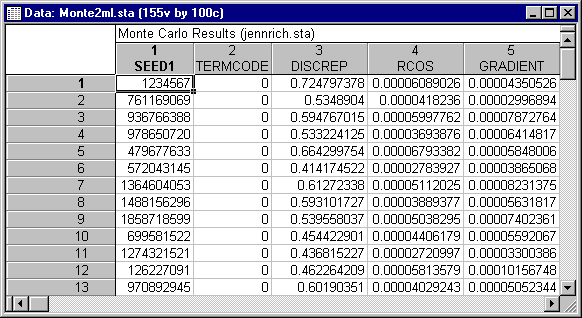
In case your computer is an older model, or your work schedule will not permit running this lengthy experiment, we have run the Monte Carlo study for you. Results from 100 replications of the ML estimation procedure are in the file Monte2ML.sta. Results on the same data for the GLS estimation procedure are in the file Monte2GL.sta. Note that your results may be slightly different, due to small differences in random number generators from earlier versions of the program; however, the conclusions obtained from this example will be the same.

Examination of these Monte Carlo results, using the data analytic facilities of STATISTICA, will provide us with some information that is relevant to the questions we addressed earlier.

Open the file Monte2ML.sta. This file contains output from 100 replications of the maximum likelihood estimation procedure.

Begin by examining the TERMCODE variable. Ideally, all termination codes should be zero, indicating that normal convergence occurred on that replication. In this case, all 100 replications converged normally.

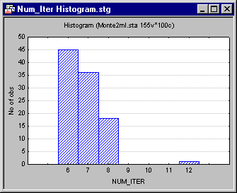
As a secondary check on the iterative process, construct a histogram of the number of iterations required for the 100 replications, and look for outliers. Click on the variable name NUM_ITER to select that variable column, and then right-click in the highlighted column to display the shortcut menu. Select Graphs of Input Data - Histogram NUM_ITER - Regular to generate the histogram illustrated below.

In this case, we find that most cases required between 7 and 9 iterations. This narrow range of low values suggests that the iterative algorithms performed in a consistent and rather stable manner on these data.

Next, examine the performance of the test statistic itself. Recall that the example was constructed to simulate a situation where the null hypothesis is, in fact, true. In this case, the test statistic has an asymptotic distribution that is central Chi-square, with 66 degrees of freedom. The question is, "How well is the asymptotic distribution approximated by the actual distribution of the test statistic in this case?"

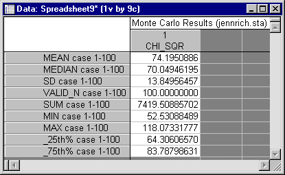
Use STATISTICA's data analytic and graphical capabilities to analyze the performance of the test statistic. First, calculate quick descriptive statistics for the CHI_SQR variable: (1) click on the variable name to select that variable column, (2) right-click in the highlighted column to display the shortcut menu, (3) select Statistics of Block Data - Block Columns - All.  

You should see the following data for the mean, 95% confidence interval endpoints, and standard deviation.

Recall that a Chi-square variable with 66 degrees of freedom should have a mean of 66, and a variance of 132, corresponding to a standard deviation of 11.489. Moreover, a Chi-square with 66 degrees of freedom has a distribution that is very close to normal in shape. Consequently, the standard (normal theory) confidence interval on the population mean should be quite accurate in this case. STATISTICA calculates the interval as ranging from 71.44 to 76.94.

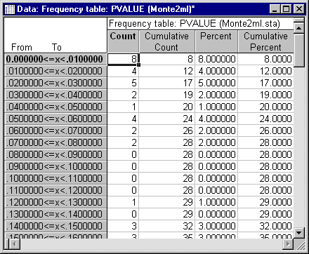
The fact that the interval excludes 66 by a wide margin indicates that the actual distribution of the Chi-square statistic clearly departs from the asymptotic distribution, and tends to have values that are too high. Moreover, the standard deviation, 13.85, is somewhat higher than the theoretical value of 11.489. These distributional characteristics would tend to lead to too frequent rejections in practice. To get some idea of the true Type I error rate for the test statistic when the nominal rate is .05, we delve further into the data by constructing a frequency distribution of the data for the variable PVALUE. PVALUE represents the probability level for the Chi-square test statistic, under the assumption that it has a central  distribution. To tell the actual proportion of Type I errors when tests are run at the a significance level, simply examine what proportion of the time the variable PVALUE has a value less than a.

In this case, we will require the services of the Basic Statistics and Tables module. Open the Monte2ML.sta data file and click on the PVALUE variable header to select that column. Select Basic Statistics/Tables from the Statistics menu to display the Basic Statistics and Tables Startup Panel.

Select Frequency tables and click OK to display the Frequency Tables dialog. Select the Advanced tab, and under Categorization method for tables & graphs, select the Step size option button and enter .01 as the value, starting at 0.0. Clear the at minimum check box. Then click the Summary: Frequency tables button. The top section of the resulting spreadsheet should contain the data shown in the following illustration. Since the total N is 100 replications, counts are identical to percentages in this case. Note that 20% of the p-values were less than .05, meaning that the actual Type I error rate was about .20 when the nominal error rate was .05.  

These data suggest that, to be considered "significant at the .05 level," values of the test statistic should have a nominal significance level less than .01. (This is based on the fact that 8% of the cases had p-values less than .01). After performing this Monte Carlo examination, the sophisticated user might well hesitate to declare the two population correlation matrices significantly different at the .05 level.

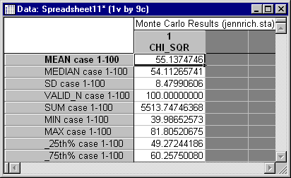
Examination of similar data for the GLS test statistic show a rather different trend. You can examine these data by opening the Monte2GL.sta data file and repeating the steps described above. The descriptive statistics show, in this case, a mean and standard deviation that are substantially lower than they should be.

Moreover, the frequency distribution for the variable PVALUE shows that there were no rejections at the .05 level. Hence, while the ML statistic is excessive, the GLS statistic is far too conservative, i.e., it rejects far too infrequently. Its conservative nature is almost certainly accompanied by very low power in this case.  

It appears that the sample size was simply too low to allow for adequate precision for the attempted analysis. Ideally, in structural modeling the number of observations should be at least 10-20 times the number of variables, and the sample sizes of 40 and 89 were just too low.  

There are probably dozens of examples of published papers employing structural equation modeling which report test statistics based on questionable sample sizes. Using Structural Equation Modeling, you can reconstruct some of these analyses, run Monte Carlo experiments, and find out for yourself how the test statistics tend to perform with particular combinations of model and sample size.

Prior analysis of system performance, using Monte Carlo methods, can inform you in advance about adequacy of sample sizes, potential convergence problems, etc. We urge you to make use of this information when using structural equation modeling in your research.

In this case, you could employ the Monte Carlo procedure to determine appropriate levels of sample size in the experiment.