Example 1: A 2 x 3 Between-Groups Factorial ANOVA Design
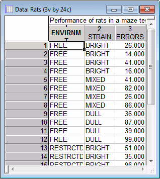
This example is based on a fictitious data set presented in Lindeman (1974). Suppose that we have conducted an experiment to address the nature vs. nurture question; specifically, we tested the performance of different rats in the "T-maze." The T-maze is a simple maze, and the rats' task is to learn to run straight to the food placed in a particular location, without errors. Three strains of rats whose general ability to solve the T-maze can be described as bright, mixed, and dull were used. From each of these strains, we reared four animals in a free (stimulating) environment and four animals in a restricted environment. The dependent measure is the number of errors made by each rat while running the T-maze problem.
Ribbon bar. Select the Home tab. In the File group, click the Open arrow and from the menu, select Open Examples. The Open a STATISTICA Data File dialog box is displayed. Rats.sta is located in the Datasets folder.
Classic menus. From the File menu, select Open Examples to display the Open a STATISTICA Data File dialog box; Rats.sta is located in the Datasets folder.
A portion of this file is shown below.
- Specifying the Analysis
- Start General Linear Models:
- Ribbon bar
- Select the Statistics tab. In the Advanced/Multivariate group, click Advanced Models and from the menu, select General Linear to display the General Linear Models (GLM) Startup Panel.
- Classic menus
- Select General Linear Models from the Statistics - Advanced Linear/Nonlinear Models submenu to display the
General Linear Models (GLM) Startup Panel.
Select Factorial ANOVA as the Type of analysis and Quick specs dialog as the Specification Method. Then click the OK button to display the GLM Factorial ANOVA Quick Specs dialog box.
In the data file Rats.sta, the codes 1-free and 2-restricted were used in the categorical predictor variable Envirnmt to denote whether the respective rat belongs to the group of rats that were raised in the free or restricted environment, respectively. You can also refer to categorical predictor variables as grouping variables, coding variables, or between-groups factors. These variables contain the codes that were used to uniquely identify to which group in the experiment the respective case belongs.
The codes used for the second categorical predictor variable (Strain) are 1-bright, 2-mixed, and 3-dull. The dependent variable in an experiment is the one that depends on or is affected by the predictor variables; in this study this would be the variable Errors, which contains the number of errors made by the respective rat running the maze.
This is a 2 (Environment) by 3 (Strain) between-groups factorial design. The variables Envirnmt and Strain are the categorical predictor variables, and variable Errors is the dependent variable. Click the Variables button on the Quick tab, specify these variables in the Dependent and Categorical predictor variable lists, and then click the OK button to return to the GLM Factorial ANOVA Quick Specs dialog box.
Next, specify the codes that were used to uniquely identify the groups; click the Factor codes button and either enter each of the codes for each variable or click the All button for each variable to enter all of the codes for that variable. Then click the OK button to return to the GLM Factorial ANOVA Quick Specs dialog box.
Now click the OK button to begin the analysis. When complete, the GLM Results dialog box is displayed.
- Results
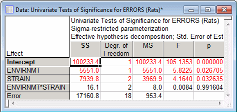
- This dialog box offers a number of output options. Click the All effects button (located on the Quick tab) to produce a spreadsheet displaying the summary ANOVA table for the analysis.
- Summary ANOVA table
- This table summarizes the main results of the analysis. Note that significant effects (p<.05) in this table are highlighted (in red) in this spreadsheet. You can adjust the significance criterion (for highlighting) by entering the desired alpha level in the Significance level field on the Quick tab. Both of the main effects (Envirnmt and Strain) are statistically significant (p<.05) while their 2-way interaction is not (p>.05).
- Reviewing marginal means
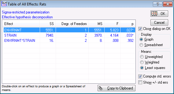
- The marginal means for the Envirnmt main effect will now be reviewed. (Note that the marginal means can be calculated as unweighted or weighted means, or as least squares means.) First, in the GLM Results dialog box, click the All effects/Graphs button to display the
Table of All Effects dialog box.
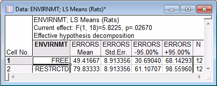
In this dialog box, select the Envirnmt main effect. In the Display group box, select the Spreadsheet option button, and then click the OK button to produce a spreadsheet with the table of marginal means for the selected effect.
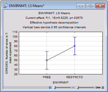
The default graph for all spreadsheets with marginal means is the means plot. In this case, the plot is rather simple. To produce this plot of the two means for the free and restricted environment, return to the Table of All Effects dialog box (by clicking the All effects/Graphs button on the Quick tab) and change the Display option to Graph, and click the OK button.
It appears that rats that were raised in the more restricted environment made more errors than the rats raised in the free environment. Now, look at all of the means simultaneously, that is, at the plot of the interaction of Environmt by Strain.
- Reviewing the interaction plot
- Once again, return to the
Table of All Effects dialog box, and select the interaction effect (Environmt*Strain). Click the OK button to display the
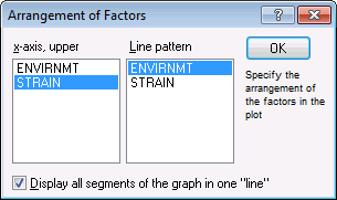
Arrangement of Factors dialog box. We have full control over the order in which the factors in the interaction will be plotted. For this example, select STRAIN in the x-axis, upper list and ENVIRNMT in the Line pattern list.
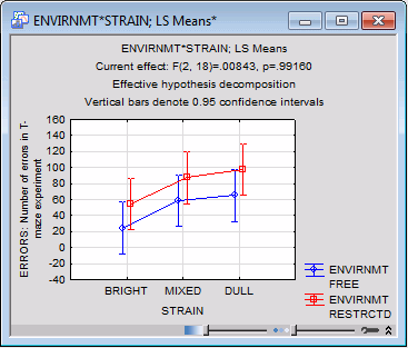
Click the OK button, and the graph of means is displayed.
The graph nicely summarizes the results of this study, that is, the two main effects pattern. The rats raised in the restricted environment (red line) made more errors than those raised in the free environment (blue line). At the same time, the dull rats made the most errors, followed by the mixed rats, and the bright rats made the fewest number of errors.
- Post Hoc Comparisons of Means
- In the previous plot, we might ask whether the mixed strain of rats was significantly different from the dull and the bright strain. However, no a priori hypotheses about this question were specified, therefore, we should use post hoc comparisons to test the mean differences between strains of rats (refer to the Introductory Overview for an explanation of the logic of post hoc tests).
- Specifying post hoc tests
- Maximize the GLM Results dialog box, and click the More results button to display the larger GLM Results dialog box. Select the Post-hoc tab. For this example, select Strain in the Effect box in order to compare the (unweighted) marginal means for that effect.
- Choosing a test
- The different post hoc tests on this tab all "protect" us to some extent against capitalizing on chance (due to the post hoc nature of the comparisons). All tests enable us to compare means under the assumption that we bring no a priori hypotheses to the study. These tests are discussed in the
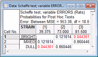
Post-hoc tab topic. For now, simply click the Scheffé test button.
This spreadsheet shows the statistical significance of the differences between all pairs of means. As we can see, only the difference between group 1 (bright) and group 3 (dull) reaches statistical significance at the p<.05 level. Thus, we would conclude that the dull strain of rats made significantly more errors than the bright strain of rats, while the mixed strain of rats is not significantly different from either.
- Testing Assumptions
- The ANOVA/MANOVA and GLM Introductory Overview - Assumptions and Effects of Violating Assumptions topic discusses the assumptions underlying the use of ANOVA techniques. These same assumptions apply to ANOVA performed using the general linear model. Now, we will review the data in terms of these assumptions.
Maximize the GLM Results dialog box, and select the Assumptions tab, which offers many different tests and graphs; some are applicable only to more complex designs.
- Distribution of dependent variable
- ANOVA assumes that the distribution of the dependent variable (within groups) follows the normal distribution. We can view the distribution for all groups combined or for only a selected group by selecting the group in the Effect drop-down box. For now, select the Environmt*Strain interaction effect, and in the Distribution of vars within groups group box, click the Histograms button. The
Select groups dialog box is first displayed, in which we can select to view the distribution for all groups combined or for only a selected group.
For this example, click the OK button to accept the default selection of All Groups, and a histogram of the distribution will be produced.
It appears as if the distribution across groups is multi-modal, that is to say, it has more than one "peak." We could have anticipated that, given the fact that strong main effects were found. If we want to test the homogeneity assumption more thoroughly, we could now look at the distributions within individual groups or plot the histograms of the within-cell residuals (deviations from the within-cell means). Instead, a potentially more serious violation of the ANOVA assumptions will be tested.
- Correlation between mean and standard deviation
- Deviation from normality is not the major "enemy" of validity of ANOVA; the most likely "trap" to fall into is to base our interpretation of an effect on an "extreme" cell in the design with much greater than average variability. Put another way, when the means and the standard deviations are correlated across cells of the design, then the performance (alpha error rate) of the F-test deteriorates greatly, and you may reject the null hypothesis with p<.05 when the real p-value is possibly as high as .50.
Now, look at the correlation between the 6 means and standard deviations in this design. We can elect to plot the means vs. either the standard deviations or the variances by clicking the appropriate button (Plot means vs. std. deviations or Variances, respectively) on the Assumptions tab. For this example, click the Plot means vs. std. deviations button.
Note: in the illustration above, a linear fit and regression bands have been added to the plot via the Graph Options - Plot: Fitting tab and the Graph Options - Plot: Regr. Bands tab. Indeed, the means and standard deviations appear substantially correlated in this design. If an important decision were riding on this study, we would be well advised to double-check the significant main effects pattern by using, for example, some nonparametric procedure (see the Nonparametrics module) that does not depend on raw scores (and variances) but rather on ranks. In any event, you should view these results with caution. - Homogeneity of variances
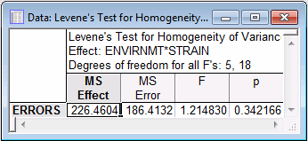
- Now, look also at the homogeneity of variance tests. On the Assumptions tab, various tests are available in the Homogeneity of variances/covariances group box. We could try a univariate test (Cochran C, Hartley, Bartlett) to compute the standard homogeneity of variances test, or the Levene's test, but neither will yield statistically significant results. Shown below is the Levene's Test for Homogeneity of Variances spreadsheet.
- Summary
- Besides illustrating the major functional aspects of the GLM module, this analysis has demonstrated how important it is to be able to graph data easily (e.g., to produce the scatterplot of means vs. standard deviations). Had we relied on nothing else but the F-tests of significance and the standard tests of homogeneity of variances, we would not have caught the potentially serious violation of assumptions that was detected in the scatterplot of means vs. standard deviations. As it stands, we would probably conclude that the effects of environment and genetic factors (Strain) both seem to have an (additive) effect on performance in the T-maze. However, the data should be further analyzed using nonparametric methods to ensure that the statistical significance (p) values from the ANOVA are not inflated.
See also GLM - Index.