Discriminant Function Analysis - Example
- Overview
- This example is based on a classic example data set reported by Fisher (1936). It contains the lengths and widths of sepals and petals of three types of irises (Setosa,
Versicol, and
Virginic). The purpose of the analysis is to learn how one can discriminate between the three types of flowers, based on the four measures of width and length of petals and sepals. In principle, all discriminant analyses address similar questions. If you are an educational researcher, you could substitute "type of flower" with "type of drop-out," and the variables (measures of sepal/petal widths and lengths) with "grades in four key courses." If you are a social scientist, you could study variables that predict people's choices of careers. In a personnel selection study, you could be interested in variables that discriminate between employees who will perform above average and will later be promoted, employees who do an adequate job, and employees who are unacceptable. Thus, even though the present example falls into the domain of biology, the general procedures shown here are generally applicable.
Specifying the Analysis.
- Data file
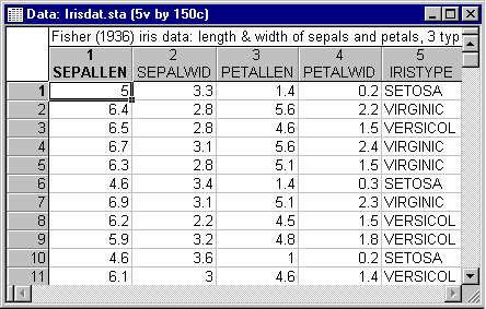
- The data file for this analysis is Irisdat.sta. A partial listing of the file is shown below. Open this data file via the File - Open Examples menu; it is in the
Datasets folder.
The first two variables in this file (Sepallen, Sepalwid) pertain to the length and width of sepals; the next two variables (Petallen, Petalwid) pertain to the length and width of petals. The last variable in this file is a grouping or coding variable that identifies to which type of iris each flower belongs (Setosa, Versicol, and Virginic). In all, there are 150 flowers in this sample, 50 of each type.
- Startup Panel
- Select Discriminant Analysis from the Statistics
- Multivariate Exploratory Techniques menu to display the Discriminant Function Analysis Startup Panel. On the
Quick tab, select the
Advanced options (stepwise analysis) check box. Click the
Variables button to display the standard variable selection dialog. Here, select
Iristype as the
Grouping variable and the remaining variables as the
Independent variable list that will be used in order to discriminate between iris types, and then click the
OK button.
Next, specify the codes that were used in the grouping variable to identify to which group each case belongs. Click the Codes for grouping variables button and either enter 1-3, click the All button, or use the asterisk (*) convention to select all codes on the Select codes for grouping variable dialog.
Click the OK button to return to the Startup Panel. Alternatively, you can click the OK button on the Startup Panel and STATISTICA will automatically search the grouping variable(s) and select all codes for those variables.
- Deletion of missing data
- This particular data file does not contain any missing data. However, if there are missing data in the file, you can either choose to ignore cases with missing data (select the Casewise option button under MD deletion) or to substitute missing data by the respective means (select the Mean substitution option button under MD deletion).
- Reviewing Descriptive Statistics
- Now click the
OK button on the Startup Panel to begin the analysis. If you have selected the Advanced options (stepwise analysis) check box on the Startup Panel, the
Model Definition dialog will be displayed, which is used to define the discriminant analysis and to review the descriptive statistics. Click on the
Descriptives tab.
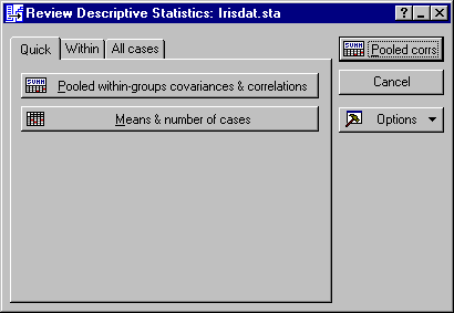
Before specifying the discriminant function analysis, click the Review descriptive stats button to look at the distribution of some of the variables and their intercorrelations. This displays the Review Descriptive Statistics dialog.
First, look at the means. On the Quick tab, click the Means & numbers of cases button to display a spreadsheet with the means and valid N for each group and for all groups combined.
- Producing a histogram from a spreadsheet
- In order to produce a histogram of the frequency distribution for a variable, first click on the desired spreadsheet column to select it. For example, to produce the histogram for variable
Sepalwid, move the cursor to the second column of the above spreadsheet. Then, right-click and select Graphs of Input Data
- Histogram Sepalwid -
Normal
Fit from the resulting shortcut menu to produce the following graph.
Many other options to graphically view the data are available on the Review Descriptive Statistics dialog. These options are described below.
- Box and whisker plot
- On the
All cases tab, click the
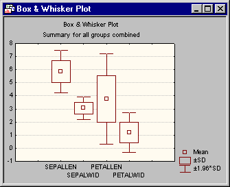
Box plot of means button to produce a box and whisker plot of the independent variables. A standard variable selection dialog is first displayed; select all of the variables and then click the
OK button. Next, the Box-Whisker Type dialog is displayed, select the Mean/SD/1.96*SD option button and then the
OK button.
This plot is useful to summarize the distribution of the variables by three components:
- A central line to indicate central tendency or location (i.e., mean or median);
- A box to indicate variability around this central tendency (i.e., quartiles, standard errors, or standard deviations);
- Whiskers around the box to indicate the range of the variable [i.e., ranges, standard deviations, 1.96 times the standard deviations (95% normal prediction interval for individual observations around the mean), or 1.96 times the standard errors of the means (95% confidence interval)].
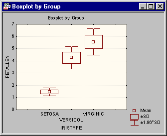
You can also view the distribution of the variables within each level of the grouping variable by clicking the Box plot of means by group button on the Within tab. Select the variable Petallen in the variable selection dialog and then click the OK button. In the Box-Whisker Type dialog, select the Mean/SD/1.96*SD option button and then click the OK button.
- Categorized histograms
- You can graphically display histograms of a variable as categorized by a grouping variable when you click the
Categorized histogram by group button on the
Within tab. When you click this button, a standard variable selection dialog is displayed in which you can select a variable from a list of the previously selected independent variables. For this example, select the variable
Sepalwid and then click the
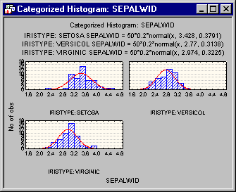
OK button. The histograms as categorized by the grouping variable selected in the Startup Panel are shown below.
As you can see, this variable is basically normally distributed within each group (type of flower).
- Scatterplots
- Another type of graph of interest would be the scatterplots of correlations between variables included in the analysis. To graphically view the correlations between variables together in a matrix scatterplot, click
Plot of total correlations button on the
All cases tab. Select all variables in the variable selection dialog and then click the
OK button.
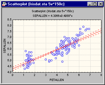
Now, look at the scatterplot for variables Sepallen and Petallen. Select Scatterplots from the Graphs menu to display the 2D Scatterplots dialog. On the Quick tab, click the Variables button and in the variable selection dialog, select Petallen as the X variable, Sepallen as the Y variable, and then click the OK button. Next, select the Confidence option button under Regression bands. Now, click the OK button.
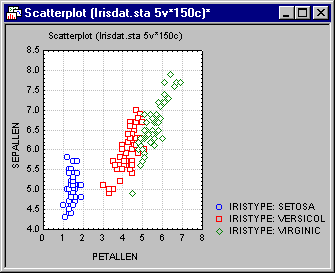
It appears that there are two "clouds" of points in this plot. Perhaps the points in the lower-left corner of this plot all belong to one iris type. If so, then there is good "hope" for this discriminant analysis. However, if not, then the possibility that the underlying distribution for these two variables is not bivariate normal, but rather multi-modal with more than one "peak," would have to be considered. To explore this possibility, create a categorized scatterplot of variables Petallen by Sepallen, categorized by Iristype. Select Scatterplots from the Graphs - Categorized Graphs menu to display the 2D Categorized Scatterplots dialog. On the Quick tab, click the Variables button to display the standard variable selection dialog. Here, select variable Petallen as the Scatterplot X, variable Sepallen as the Scatterplot Y, variable Iristype as the X-Category, and then click the OK button. Also, click the Overlaid option button under Layout and then click the OK button on the 2D Categorized Scatterplots dialog to produce the following plot.
This scatterplot shows the correlation between variables Sepallen and Petallen within groups. Thus, it can be concluded that the assumption of a bivariate normal distribution within each group is probably not violated for this particular pair of variables.
- Specifying Discriminant Function Analysis
- Now, return to the primary goal of the analysis; click the
Cancel button on the
Review Descriptive Statistics dialog to return to the
Model Definition dialog. Perform a stepwise analysis in order to see what happens at each step of the discriminant analysis. On the
Advanced tab, select
Forward stepwise in the
Method box. In this setting, STATISTICA will enter variables into the discriminant function model one by one, always choosing the variable that makes the most significant contribution to the discrimination.
Stop rules. STATISTICA will keep "stepping" until one of four things happen. The program will terminate the stepwise procedure when:
- All variables have been entered or removed, or
- The maximum number of steps has been reached, as specified in the Number of steps box, or
- No other variable that is not in the model has an F value greater than the F to enter that is specified in this dialog and when no other variable in the model has an F value that is smaller than the F to remove specified in this dialog, or
- Any variable after the next step would have a tolerance value that is smaller than that specified in the Tolerance box.
- F to enter/remove
- When stepping forward, STATISTICA will select the variable for inclusion that makes the most significant unique (additional) contribution to the discrimination between groups; that is, STATISTICA will choose the variable with the largest F value (greater than the respective user-specified
F to enter value). When stepping backward, STATISTICA will select the variable for exclusion that is least significant, that is, the variable with the smallest F value (less than the respective user-specified
F to remove value). Therefore, if you want to enter all variables in a forward stepwise analysis, set the
F to enter value as small as possible (and the
F to remove to 0).
If you want to remove all variables from a model, one by one, set F to enter to a very large value (e.g., 9999), and also set F to remove to a very large value that is only marginally smaller than the F to enter value (e.g., 9998). Remember that the F to enter value must always be set to a larger value than the F to remove value.
- Tolerance
- The meaning of the
Tolerance value was introduced in the
Introductory Overviews. In short, at each step STATISTICA will compute the multiple correlation (R-square) for each variable with all other variables that are currently included in the model. The tolerance value of a variable is then computed as 1 minus R-square. Thus, the tolerance value is a measure of the redundancy of a variable.
For example, if a variable that is about to enter into the model has a tolerance value of .01, then this variable can be considered to be 99% redundant with the variables already included. At one point, when one or more variables become too redundant, the variance-/covariance matrix of variables included in the model can no longer be inverted, and the discriminant function analysis cannot be performed.
It is generally recommended that you leave the Tolerance setting at its default value of 0.01. If a variable is included in the model that is more than 99% redundant with other variables, then its practical contribution to the improvement of the discriminatory power is dubious. More importantly, if you set the tolerance to a much smaller value, round-off errors may result, leading to unstable estimates of parameters.
- Starting the analysis
- After reviewing the different options on this dialog, you can proceed in the usual manner, that is, do not change any of the default settings for now. However, in order to view the results of the analyses at each step, change the
Display results box to At each step. Now, click the
OK button to begin the discriminant analysis.
Reviewing the Results of Discriminant Analysis.
Results at Step 0. First, the Discriminant Function Analysis Results dialog at Step 0 is displayed. Step 0 means that no variable has yet been included into the model.
Because no variable has been entered yet, most options on this dialog are not yet available (i.e., they are dimmed). However, you can review the variables not in the equation via the Variables not in the model button.
- Wilks' lambda
- In general, Wilks' lambda is the standard statistic that is used to denote the statistical significance of the discriminatory power of the current model. Its value will range from 1.0 (no discriminatory power) to 0.0 (perfect discriminatory power). Each value in the first column of the spreadsheet shown above denotes the Wilks' lambda after the respective variable is entered into the model.
- Partial Wilks' lambda
- This is the
Wilks' lambda for the unique contribution of the respective variable to the discrimination between groups. In a sense, one can look at this value as the equivalent to the partial correlation coefficients reported in Multiple Regression. Because a
lambda of 0.0 denotes perfect discriminatory power, the lower the value in this column, the greater is the unique discriminatory power of the respective variable. Because no variable has been entered into the model yet, the
Partial Wilks' lambda at step 0 is equal to the
Wilks' lambda after the variable is entered, that is, the values reported in the first column of the spreadsheet.
F to enter and p-value. Wilks' lambda can be converted to a standard F value (see Notes), and you can compute the corresponding p-values for each F. However, as discussed in the Introductory Overviews, one should generally not take these p-values at face value. One is always capitalizing on chance when including several variables in an analysis without having any a priori hypotheses about them, and choosing to interpret only those that happen to be "significant" is not appropriate.
In short, there is a big difference between predicting a priori a significant effect for a particular variable and then finding that variable to be significant, as compared to choosing from among 100 variables in the analysis the one that happens to be significant. Without going into details, in purely practical terms, in the latter case, it is not very likely that you would find the same variable to be significant if you were to replicate the study. When reporting the results of a discriminant function analysis, you should be careful not to leave the impression as if only the significant variables were chosen in the first place (for some theoretical reasons), when, in fact, they were chosen because they happened to "work."
Looking at the spreadsheet above, you can see that the largest F to enter is shown for variable Petallen. Thus, that variable will be entered into the model at the next (first) step.
- Tolerance and R-square
- The Tolerance value was discussed earlier in this section (refer also to the Introductory Overviews); to reiterate, it is defined as 1 minus R-square of the respective variable with all other variables in the model, and this value gives an indication of the redundancy of the respective variable. Since no other variables have been chosen yet, all R-squares are equal to 1.0.
- Results at Step 2
- Now, click the
Next button to go to the next step. Step 1 will not be discussed here, so click the
Next button again to go to
Step 2 (the model with 2 variables). The
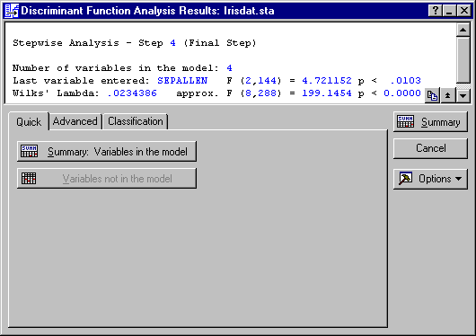
Discriminant Function Analysis Results dialog will look like this.
Overall, the discrimination between types of irises is highly significant (Wilks' Lambda = .037; F = 307.1, p<0.0001). Now look at the independent contributions to the prediction for each variable in the model.
- Variables in the model
- Click the Summary: Variables in the model button to display the spreadsheet of results for the variables currently in the model. As you can see, both variables are highly significant.
- Variables not in the model
- Now click the
Variables not in the model button to display a spreadsheet with the same statistics that were reviewed earlier.
As you can see, both variables that are not yet in the model have F to enter values that are larger than 1; thus, you know that the stepping will continue and that the next variable that will enter into the model is the variable Petalwid.
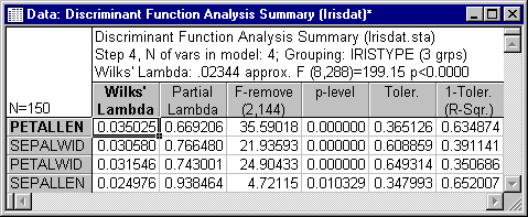
Results at Step 4 (Final Step).
Once again, click the Next button in the Discriminant Function Analysis Results dialog to go to the next step in the analysis. Step 3 will not be reviewed here, so click the Next button again to go to the final step in the analysis - Step 4.
Now, click the Summary: Variables in the model button to review the independent contributions for each variable to the overall discrimination between types of irises.
The Partial Wilks' Lambda indicates that variable Petallen contributes most, variable Petalwid second most, variable Sepalwid third most, and variable Sepallen contributes least to the overall discrimination. (Remember that the smaller the Partial Wilks' Lambda, the greater is the contribution to the overall discrimination.) Thus, you may conclude at this point that the measures of the petals are the major variables that allow you to discriminate between different types of irises. To learn more about the nature of the discrimination, you need to perform a canonical analysis. Thus, click on the Advanced tab.
- Canonical Analysis
- Next, compute the actual discriminant functions to see how the four variables discriminate between the different groups (types of irises). Click the
Perform canonical analysis button to perform the canonical analysis and open the
Canonical Analysis dialog.
As discussed in the Introductory Overviews, STATISTICA will compute different independent (orthogonal) discriminant functions. Each successive discriminant function will contribute less to the overall discriminatory power. The maximum number of functions that is estimated is either equal to the number of variables or the number of groups minus one, whichever number is smaller. In this case, two discriminant functions will be estimated.
- Significance of roots
- First, determine whether both discriminant functions (roots) are statistically significant. Click the
Summary: Chi square test of successive roots button and the following spreadsheet is displayed.
In general, this spreadsheet reports a step-down test of all canonical roots. The first line always contains the significance test for all roots; the second line reports the significance of the remaining roots, after removing the first root, and so on. Thus, this spreadsheet tells you how many canonical roots (discriminant functions) to interpret. In this example, both discriminant (or canonical) functions are statistically significant. Thus, you will have to come up with two separate conclusions (interpretations) of how the measures of sepals and petals allow you to discriminate between iris types.
- Discriminant function coefficients
- Click the
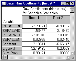
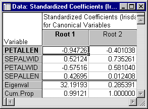
Coefficients for canonical variables button. Two spreadsheets are produced, one for the
Raw Coefficients and one for the Standardized Coefficients. Now, look at the
Raw Coefficients spreadsheet.
Raw here means that the coefficients can be used in conjunction with the observed data to compute (raw) discriminant function scores. The standardized coefficients are the ones that are customarily used for interpretation, because they pertain to the standardized variables and therefore refer to comparable scales.
The first discriminant function is weighted most heavily by the length and width of petals (variable Petallen and Petalwid, respectively). The other two variables also contribute to this function. The second function seems to be marked mostly by variables Sepalwid, and to a lesser extent by Petalwid and Petallen.
- Eigenvalues
- Also shown in the spreadsheet above are the Eigenvalues (roots) for each discriminant function and the Cumulative Proportion of explained variance accounted for by each function. As you can see, the first function accounts for over 99% of the explained variance; that is, 99% of all discriminatory power is explained by this function. Thus, this first function is clearly the most "important" one.
- Factor structure coefficients
- These coefficients (which can be viewed via the
Factor structure button on the
Canonical Analysis - Advanced tab) represent the correlations between the variables and the discriminant functions and are commonly used in order to interpret the "meaning" of discriminant functions (see also the discussion in the Introductory Overviews).
In educational or psychological research it is sometimes desired to attach meaningful labels to functions (e.g., "extroversion," "achievement motivation"), using the same reasoning as in factor analysis (see Factor Analysis). In those cases, the interpretation of factors should be based on the factor structure coefficients. However, such meaningful labels for these functions will not be considered for this example.
- Means of canonical variables
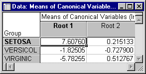
- You now know how the variables participate in the discrimination between different types of irises. The next question is to determine the nature of the discrimination for each canonical root. The first step to answer this question is to look at the canonical means. Click the
Means of canonical variables button on the
Advanced tab.
Apparently, the first discriminant function discriminates mostly between the type Setosa and the other iris types. The canonical mean for Setosa is quite different from that of the other groups. The second discriminant function seems to distinguish mostly between type Versicol and the other iris types; however, as one would expect based on the review of the eigenvalues earlier, the magnitude of the discrimination is much smaller.
- Scatterplot of canonical scores
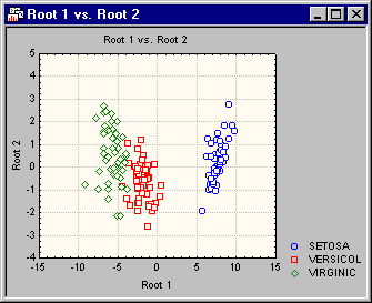
- A quick way of visualizing these results is to produce a scatterplot for the two discriminant functions. Click on
Canonical Analysis - Canonical Scores tab and then click the
Scatterplot of canonical scores button to plot the unstandardized scores for
Root 1 vs.
Root 2.
This plot confirms the interpretation so far. Clearly, the flowers of type Setosa are plotted much further to the right in the scatterplot. Thus, the first discriminant function mostly discriminates between that type of iris and the two others. The second function seems to provide some discrimination between the flowers of type Versicol (which mostly show negative values for the second canonical function) and the others (which have mostly positive values). However, the discrimination is not nearly as clear as that provided by the first canonical function (root).
- Summary
- To summarize the findings so far, it appears that the most significant and clear discrimination is possible for flowers of type Setosa by the first discriminant function. This function is marked by negative coefficients for the width and length of petals and positive weights for the width and length of sepals. Thus, the longer and wider the petals, and the shorter and smaller the sepals, the less likely it is that the flower is of iris type Setosa (remember that in the scatterplot of the canonical functions, the flowers of type Setosa were plotted to the right, that is, they were distinguished by high values on this function).
- Classification
- Now, return to the Discriminant Function Analysis Results dialog (click the Cancel button on the Canonical Analysis dialog) and turn to the problem of classification. As discussed in the Introductory Overviews, one goal of a discriminant function analysis is to enable the researcher to classify cases. Now, see how well the current discriminant functions classify the flowers.
- Classification Functions
- First look at the classification functions. As described in the Introductory Overview, these are not to be confused with the discriminant functions. Rather, the classification functions are computed for each group and can be used directly to classify cases. You would classify a case into the group for which it has the highest classification score. Click on the
Discriminant Function Analysis Results - Classification
tab and then click the
Classification functions button to see those functions.
You could use these functions to define the transformations for three new variables. As you would then enter new cases, STATISTICA would automatically compute the classification scores for each group.
- A priori Probabilities
- As discussed in the
Introductory Overviews, you can specify different
a priori probabilities for each group (by using the
User defined option button under
A priori classification probabilities on the
Classification
tab). These are the probabilities that a case belongs to a respective group, without using any knowledge of the values for the variables in the model. For example, you may know
a priori that there are more flowers of type
Versicol in the world, and therefore, the
a priori probability of a flower to belong to that group is higher than that for any other group. A priori probabilities can greatly affect the accuracy of the classification. You can also compute the results for selected cases only (by using the
Select button). This is particularly useful if you want to validate the discriminant function analysis results with new additional data. However, for this example, simply accept the default selection of the
Proportional to group sizes option button.
Classification Matrix. Now, click the Classification matrix button. In the resulting spreadsheet, the second line in each column header indicates the a priori classification probabilities.
Because there were exactly 50 flowers of each type, and you chose those probabilities to be proportional to the sample sizes, the a priori probabilities are equal to 1/3 for each group. In the first column of the spreadsheet, you see the percent of cases that are correctly classified in each group by the current classification functions. The remaining columns show the number of cases that are misclassified in each group, and how they are misclassified.
- A priori versus post hoc classification
- As discussed in the
Introductory Overviews, when classifying cases from which the discriminant functions were computed, you usually obtain a fairly good discrimination (although usually not as good as in this example). However, you should only look at those classifications as a diagnostic tool for identifying areas of strengths and weaknesses in the current classification functions, because these classifications are not
a priori predictions but rather
post hoc classifications. Only if you classify different (new) cases can you interpret this table in terms of predictive discriminatory power. Thus, it would be unjustified to claim that you can successfully predict the type of iris in 98 percent of all cases, based on only four measurements. Because you capitalized on chance, you could expect much less accuracy if you were to classify new cases (flowers).
Classification of Cases.
- Mahalanobis distances and posterior probabilities
- Now, return again to the
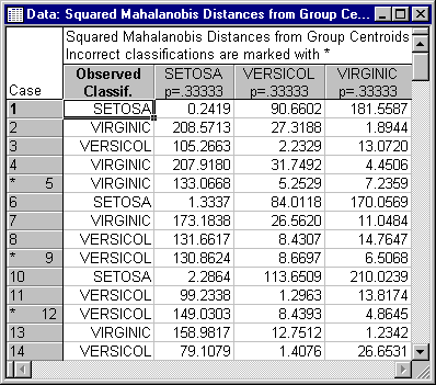
Results dialog. As described in the Introductory Overviews, cases are classified into the group to which they are closest. The Mahalanobis distance is a measure of the distance that can be used in the multivariate space defined by the variables in the model. You can compute the distance between each case and the center of each group (i.e., the group centroid, defined by the respective group means for each variable). The closer the case is to a group centroid, the more confidence you can have that it belongs to that group. Mahalanobis distances can be computed by clicking the
Squared Mahalanobis distances button on the
Classification tab. Shown below is part of the
Squared Mahalanobis Distances from Group Centroids spreadsheet.
You can also directly compute the probability that a case belongs to a particular group. This is a conditional probability, that is, it is contingent on your knowledge of the values for the variables in the model. Thus, these probabilities are called posterior probabilities. You can request those probabilities via the Posterior probabilities button. Note that as in the case of the classification matrix, you can select cases to be classified, and you can specify different a priori probabilities.
- Actual classifications
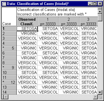
- Shown below is a partial listing of the actual classifications of cases (flowers; click the
Classification of cases button).
The classifications are ordered into a first, second, and third choice. The column under the header 1 contains the first classification choice, that is, the group for which the respective case had the highest posterior probability. The rows marked by the asterisk (*) are cases that are misclassified. Again, in this example, the classification accuracy is very high, even considering the fact that these are all post hoc classifications. Such accuracy is rarely attained in research in the social sciences.
- Summary
- This example illustrates the basic ideas of discriminant function analysis. In general, in many cases where there are naturally occurring groups that you would like to be able to discriminate, this technique is appropriate. However, as stated at various points in the preceding discussion, if correct predictive classification is the goal of the research, then at least two studies must be conducted: one in order to build the classification functions and another to validate them.
See also, Discriminant Function Analysis - Index.

