Fitting a Trend Line for Linearly Dependent Data Values
Linear regression is the statistical fitting of a trend line to an observed dataset, in which one of the data values - the dependent variable - is found to be linearly dependent on the value of the other causal data values or variables - the independent variables.
- The dependent variable is sometimes called the prediction, and the independent variables the predictors.
- The Team Studio Linear Regression operator is the simplest and one of the most frequently used modeling operators. For information about configuring these operators, see Linear Regression (DB) or Linear Regression (HD).
- Typically, a linear regression should be the first method attempted for determining the relationship between a continuous, numeric variable and a set of causal variables before any more complex methods are tried.
Linear regression is an approach to modeling the relationship between a dependent variable Y and one or more explanatory, or predictor, variables denoted X. If there is a linear association, a change in X has a corresponding change in Y. This relationship is analyzed and estimated in the form of a Linear Regression equation, such as

 act as scaling factors.
In other words, Linear Regression is the statistical fitting of a trend line to an observed dataset, in which one of the data values is found to be dependent on the value of the other data values or variables.
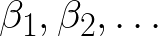
Example of simple linear regression with only one explanatory variable X.
Single variable or Simple Linear Regression is easy to understand since it can be represented as trying to best fit a line to an XY dataset, as illustrated above.
The case where only one explanatory variable X is involved is called Simple Linear Regression. Single variable or Simple Linear Regression can be represented as trying to best fit a line to a XY dataset. When a dataset has more than one independent variable involved, it is called Multivariate Linear Regression (MLR). The algebra behind a Multivariate Linear Regression Equation for predicting the Dependent Variable Y as related to the Independent Variables X can be generically expressed in the following form:


The
Team Studio Linear Regression operator runs an algorithm on the
XY dataset to determine the best fit values for the Intercept constant,
 , and Coefficient values,
 .
.
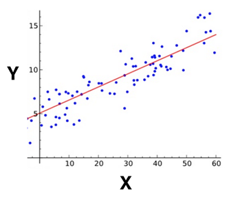
There are various ways to estimate such a best fit linear equation for a given dataset. One of the most commonly used methods, also used by the Team Studio Linear Regression Algorithm, is the ordinary least-squares (OLS) approach. This method calculates the best-fitting line for the observed data by minimizing the sum of the squares of the vertical deviations of each data point to the line (if a point lies on the fitted line exactly, then its vertical deviation is 0). Because the deviations are first squared, then summed, there are no cancellations between positive and negative values.
The following diagram depicts this concept of minimizing the squares of the deviations, d, of the data points from the linear regression.
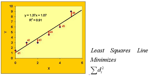
Illustration of the Ordinary Least Squares Method of Linear Regression Estimation1
Also calculated during the least-squares method is a Correlation Coefficient, R, which varies between -1 and +1.
where are the line data values and are the actual data values.
The square of the correlation coefficient, R2, is useful for understanding how well a linear equation fits the analyzed dataset. R2 represents the fraction of the total variance explained by regression. This statistic is equal to one if the fit is perfect, and to zero when the data shows no linear explanatory power whatsoever.
For example, if the R2 value is 0.91, 91% of the variance in Y is explained by the regression equation.
- Regularization of Linear Regression
-
The Ordinary Least Squares approach sometimes results in highly variable estimates of the regression coefficients, especially when the number of predictors is large relative to the number of observations. To avoid the problem of over-fitting the Regression model, especially when there is not a lot of data available, adding a regularization parameter (or constraint) to the model can help reduce the chances of the coefficients being arbitrarily stretched due to data outliers. Regularization refers to a process of introducing additional information in order to prevent over-fitting, usually in the form of a penalty or constraint for data complexity.
Three common implementations of Linear Regression Regularization include Ridge, Lasso, and Elastic Net Regularization.
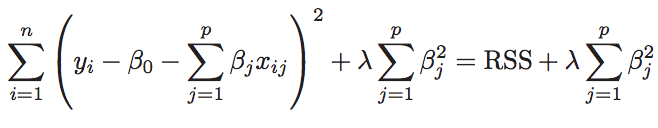
- L2 Regularization (Ridge)
-
Minimizes the quantity above. The coefficients shrink towards zero, although they never become exactly zero. Ridge constrains the sum of squares of the coefficients in the loss function. L2 Regularization results in a large number of non-zero coefficients.
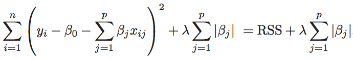
- L1 Regularization (Lasso)
-
Minimizes the quantity above. The coefficients shrink toward zero, with some coefficients becoming exactly zero to help with variable selection. Lasso constrains the sum of the absolute values of the coefficients in the loss function. L1 Regularization gives sparse estimates. Namely, in a high dimensional space, many of the resulting coefficients are zero. The remaining non-zero coefficients weigh the explanatory variable(s) (X) found to have importance in determining the dependent variable, Y.
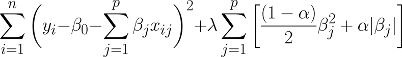
- Elastic Net Regularization
-
Combines the effects of both the Ridge and Lasso penalty constraints in the loss function given by:
If Elastic Parameter α = 1, the loss function becomes L1 Regularization (Lasso) and if α = 0, the loss function becomes L2 Regularization (Ridge). When α is between 0~1, the loss function implements a mix of both L1 (Lasso) and L2 (Ridge) constraints on the coefficients.
With higher lambda, the loss function penalizes the coefficients except the intercept. As a result, with really large lambda in linear regression, the coefficients are all zero, and the intercept is the average of the response. Logistic regression has a similar property, but the intercept is understood as prior-probability.
In general, use regularization to avoid overfitting, so multiple models with different lambda should be trained, and the model with smallest testing error should be chosen. Try lambda with values from [0, 0.1, 0.2, 0.3, 0.4, ... 1.0].
- Linear Regression Use Case (1)
The following use case analyzes a United Nations dataset with sample Education, Literacy, Life Expectancy and GDP data. - Linear Regression Use Case (2)
This use case overviews the analysis of the linear relationship between the compressive strength of concrete and varying amounts of its components, especially cement.