Linear Regression (DB)

Information at a Glance

Category	Model
Data source type	DB
Sends output to other operators	Yes
Data processing tool	n/a

Note: The Linear Regression (DB) operator is for database data only. For Hadoop data, use the Linear Regression (HD) operator.

For more information about using linear regression, see Fitting a Trend Line for Linearly Dependent Data Values.

Algorithm

The Team Studio Linear Regression operator applies a Multivariate Linear Regression (MLR) algorithm to the input data set. For MLR, a Regularization Penalty Parameter that can be applied in order to prevent of the chances of over-fitting the model.

The Linear Regression operator implements Ordinary Regression and allows for the Stepwise Feature to avoid over-fitting a model with too many variables. The Ordinary Regression algorithm uses the Ordinary Least Squares (OLS) method of regression analysis, meaning that the model is fit such that the sum-of-squares of differences of observed and predicted values is minimized.

Input

A data set that contains the dependent and independent variables for modeling.

Configuration

Parameter	Description
Notes	Any notes or helpful information about this operator's parameter settings. When you enter content in the Notes field, a yellow asterisk is displayed on the operator.
Dependent Column	The dependent column specified for the regression. This is the quantity to model or predict. The list of the available data columns for the Regression operator is displayed. Select the data column to consider the dependent variable for the regression. The Dependent Column should be a numerical data type.
Columns	Click Select Columns to select the available columns from the input data set for analysis. For a linear regression, select the independent variable data columns for the regression analysis or model training. You must select at least one column or one interaction variable.
Interaction Parameters	Enables selecting available independent variables, where those data parameters might have a combined effect on the dependent variable. See Interaction Parameters Dialog box for detailed information.
Stepwise Feature Selection	true implements stepwise regression methodology. Selecting true means that one of the possible Stepwise Type regression methods is used and the Criterion Type and Check Value must be specified. The Stepwise Feature allows the system to find a subset of variables that works just as well as the larger, original variable set. A smaller model is generally considered by data scientists to be safer from the danger of overfitting a model with too many variables. false (the default) specifies that all the independent variables specified in Column Names and Interaction Columns are considered at once when running the regression analysis and included in the model.
Stepwise Type	Specifies the different ways to determine which of the independent variables are the most predictive to include in the model. This option is enabled only if Stepwise Feature Selection is selected. For all Stepwise Type methods, the minimum significance value is defined by the operator's Check Value parameter specified, and the approach for determining the significance is defined by Criterion Type. FORWARD - (The default.) For a Forward Regression analysis process, the feature selection begins with no variables in the model and adds one variable at a time. Each potential independent variable's contribution to the model is calculated individually. The most significant variable - as defined by the approach selected for Criterion Type - is first added to the model. This process is repeated until none of the remaining unused variables meets a minimum significance level. After a variable is included it remains in the model. Note: Use this method if there is a large set of variables and you suspect that only a few of them are needed. BACKWARD - For a Backward Regression analysis process, the feature selection begins with all variables included in the model. The significance of the variables is calculated and the variable with the least significance - as defined by the approach selected for Criterion Type - is removed from the model. The process is repeated until the least significant variable meets a minimum significance level. Use this method if you are starting with a small set of variables and only a few need to be eliminated. STEPWISE For a stepwise regression analysis process, the same FORWARD method steps are taken, except that after a variable is added to the model, the included variables are re-evaluated for significance. If an included variable no longer meets the significance criteria, it is removed from the model. Feature selection of variables to include terminates when none of the remaining variables meet the selection criteria or the last variable to be included has also just been removed. This is the most powerful and typically used Stepwise Type.
Criterion Type	Specifies the approach for evaluating a variable's significance in the regression model. Enabled only if Stepwise Feature Selection is selected. AIC - The popular Akaike Information Criterion (AIC) is a specific measure of the relative goodness of fit of a statistical model. Selecting this criterion type applies a function of the number of features or variables included and the maximized likelihood function for the model. SBC - The Schwarz Bayesian Information Criterion (SBC) is similar to the AIC significance function but includes a larger penalty term for the number of selected features - that is, included variables. Choose SBC to prevent over-fitting of a model by not taking on too many variables.
Check Value	Specifies the minimal significance level value to use as feature selection criterion in Forward, Backward, or Stepwise Regression Analysis. Enabled only if Stepwise Feature Selection is selected. Default value: 0.05. If you are running without a stepwise approach, consider setting Check Value to 10% of the resulting AIC value.
Group By	Specifies a column for categorizing or subdividing the model into multiple models based on different groupings of the data. A typical example is using gender to create two different models based on the data for males versus females. A modeler might do this to determine if there is a significant difference in the correlation between the dependent variable and the independent variable based on whether the data is for a male or a female. The Group By column cannot be selected as a Dependent Column or as an independent variable (in Columns in the model.
Draw Residual Plot	Provides the option to output Q-Q Plot and Residual Plot graphs for the linear regression results. See Output for details on the resulting output graphs when Draw Residual Plot is set to true. Default value: false.

Output

Visual Output

Ordinary Linear Regression Output

Because data scientists expect model prediction errors to be unstructured and normally distributed, the Residual Plot and Q-Q Plot together are important linear regression diagnostic tools, in conjunction with R2, Coefficient and P-value summary statistics.

The remaining visual output consists of Summary, Data, Residual Plot, and Q-Q Plot.

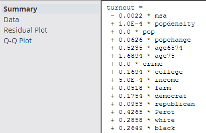
Summary

The Summary output displays the details of the derived linear regression model's Equation and Correlation Coefficient values along with the R2 and Standard Error statistical values.

The derived linear regression model is shown as a mathematical equation linking the Dependent Variable (Y) to the independent variables (X1, X2, etc.). It includes the scaling or Coefficient values (β1, β2, etc.) associated with each independent variable in the model.

Note: The resulting linear equation is expressed in the form of Y= β0 + β1*X1 + β2*X2 + ….

The following overall model statistical fit numbers are displayed.

R2: it is called the multiple correlation coefficient of the model, or the Coefficient of Multiple Determination. It represents the fraction of the total Dependent Variable (Y) variance explained by the regression analysis, with 0 meaning 0% explanation of Y variance and 1 meaning 100% accurate fit or prediction capability.
Note: in general, an R2 value greater than .8 is considered a good model. However, this value is relative and in some situations just getting an improved R2 from .5 to .6, for example, would be beneficial.
S: represents the standard error per model (often also denoted by SE). It is a measure of the average amount that the regression model equation over-predicts or under-predicts.
The rule of thumb data scientists use is that 60% of the model predictions are within +/- 1 SE and 90% are within +/- 2 SEs.

For example, if a linear regression model predicts the quality of the wine on a scale between 1 and 10 and the SE is .6 per model prediction, a prediction of Quality=8 means the true value is 90% likely to be within 2*.6 of the predicted 8 value (that is, the real Quality value is likely between 6.8 and 9.2).

In summary, the higher the R2 and the lower the SE, the more accurate the linear regression model predictions are likely to be.

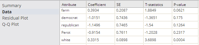
Data

The Data results are a table that contains the model coefficients and statistical fit numbers for each independent variable in the model.

Column	Description
Coefficient	The model coefficient, β, indicates the strength of the effect of the associated independent variable on the dependent variable. In the case where L1 Regularization is applied (α > 0), if the resulting coefficient value is 0 it typically means that this variable is much less relevant to the model (assuming that normalization of the variables was performed beforehand).
SE	Standard Error, or SE, represents the standard deviation of the estimated coefficient values from the actual coefficient values for the set of variables in the regression. It is best practice to commonly expect + or - 2 standard errors, meaning the actual coefficient value should be within 2 SEs of the estimate. Therefore, a modeler looks for the SE values to be much smaller than the associated forecasted coefficient values.
T-statistic	The T-statistic is computed by dividing the estimated value of the β Coefficient by its Standard Error, as follows: T= β/SE. It provides a scale for how big of an error the estimated coefficient has. A small T-statistic alerts the modeler to the fact that the error is almost as big as the coefficient measurement and is therefore suspicious. The larger the absolute value of T, the less likely that the unknown actual value of the coefficient could be zero.
P-value	The P-value represents the probability of still observing the dependent variable's value if the coefficient value for the independent variable is zero (that is, if p-value is high, the associated variable is not considered relevant as a correlated, independent variable in the model). A low P-value is evidence that the estimated coefficient is not due to measurement error or coincidence, and therefore, is more likely a significant result. Thus, a low P-value gives the modeler confidence in the significance of the variable in the model. Standard practice is to not trust coefficients with P-values greater than 0.05 (5%). Note: Note: A P-value of less than 0.05 is often conceptualized as there being over 95% certainty that the coefficient is relevant. The smaller the P-value, the more meaningful the coefficient or the more certainty over the significance of the independent variable in the linear regression model. In summary, when assessing the Data tab results of the Linear Regression operator, a modeler mostly cares about the coefficient values, which indicate the strength of the effect of the independent variables on the dependent variable, and the associated P-values, which indicate how much not to trust the estimated correlation measurement.

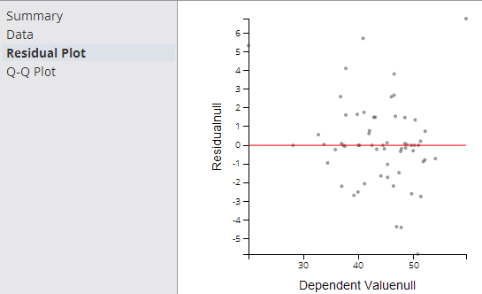
Residual Plot

The Residual Plot displays a graph that shows the residuals (differences between the observed values of the dependent variable and the predicted values) of a linear regression model on the vertical axis and the independent variable on the horizontal axis, as shown in the following example.

A modeler should always look at the Residual Plot as it can quickly detect any systematic errors with the model that are not necessarily uncovered by the summary model statistics. It is expected that the Residuals of the dependent variable vary randomly above and below the horizontal access for any value of the independent variable.

If the points in a residual plot are randomly dispersed around the horizontal axis, a linear regression model is appropriate for the data; otherwise, a non-linear model is more appropriate.

A "bad" Residual Plot has some sort of structural bend or anomaly that cannot be explained away. For example, when analyzing medical data results, the linear regression model might show a good fit for male data but have a systematic error for female data. Glancing at a Residual Plot could quickly catch this structural weakness with the model.

In summary, the Residual Plot is an important diagnostic tool for analyzing linear regression results, allowing the modeler to keep a hand in the data while still analyzing overall model fit.

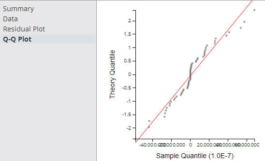
Q-Q Plot

The Q-Q (Quantile-Quantile) Plot graphically compares the distribution of the residuals of a given variable to the normal distribution (represented by a straight line), as shown in the following example.

The closer the dots are to the line, the more normal of a distribution the data has. This provides a better sense of whether a linear regression model is a good fit for the data. Any sort of variance from the line for a certain quantile, or section, of data should be investigated and understood.

The Q-Q Plot is an interesting analysis tool, although not always easy to read or interpret.

Data Output

A file with structure similar to the visual output structure is available.

Contents