Attribute Gage Study (Analytic Method) - Computational Details
This section provides the computational details and the formulas that were used in the implementation of the Attribute Gage Study (Analytic Method) in this module.
Probability plot
The Attribute Gage Study (Analytic Method) Summary plot includes a probability plot for the given reference values. This plot includes a least squares regression line that examines the relationship between the probability of acceptances (Z-scores) and the reference values of the measured parts.
Fitted line
The general form of the fitted line is:
Y = b0 + b1 X
where b0 is the intercept
b1 is the slope (the slant of the regression line), and
X is the predictor value.
R-square for fitted line
The r-square for fitted line is the coefficient of determination, which measures the reduction in the total variation of the dependent variable (i.e., probability of acceptance) due to the independent variable (such as reference values). It represents the proportion of variation in probability of acceptance that is explained by the regression model.
R-square = 1 - [Residual SS/Total SS]
Where Residual SS is the error sums of squares and the Total SS is the total sums of squares.
Gage study statistics
The following statistics are displayed in the Data statistics spreadsheet and in the Summary plot.
Bias
Bias is the difference between the actual measurement and the given reference value. When the actual measurement is unknown, the Attribute Gage Study (Analytic Method) estimates the bias as a function of either the lower tolerance limit or the upper tolerance limit.
Bias with lower limit
When a lower tolerance limit is given, the estimated bias is
LL + b0 / b1
where
LL is the lower tolerance limit,
b0 is the intercept of the fitted regression line
and b1 is the slope of the fitted regression line.
Bias with upper limit
When an upper tolerance limit is given, the estimated bias is
UL + b0 / b1
where
UL is the upper tolerance limit,
b0 is the intercept of the fitted regression line
and b1 is the slope of the fitted regression line.
Unadjusted repeatability
The unadjusted repeatability is calculated as:
where
XT (Pa 0.995) is the estimated reference value or the percentile at the 0.995 probability of acceptance from the fitted line, and
XT (Pa 0.005) is the estimated reference value or the percentile at the 0.005 probability of acceptance from the fitted line.
Adjusted repeatability
The adjusted repeatability is calculated as:
where
XT (Pa 0.995) is the estimated reference value or the percentile at the 0.995 probability of acceptance from the fitted line, and
XT (Pa 0.005) is the estimated reference value or the percentile at the 0.005 probability of acceptance from the fitted line.
The denominator, 1.08, is the adjustment factor given by AIAG, 2002. The adjusted repeatability value is used to test bias = 0.
AIAG Method
When the AIAG method is used to test the null hypothesis of bias = 0, the following statistics are calculated and reported. See AIAG, 2002 for more information.
T
To test bias = 0 using the AIAG method, the following formula for t is used:
where:
bias is calculated as given above
AR is the adjusted repeatability as given above.
The values 31.3 and 1.08 (in the formula for adjusted repeatability) are simulation results specific to the case when you have 20 trials for all parts and:
6 parts have acceptances greater than 0 and less than 20
1 part has 0 acceptances
1 part has 20 acceptances
p-value
The p-value for the AIAG test statistic, T, taken from a Student’s t distribution with 19 degrees of freedom.
Regression Method
When the regression method is used to test the null hypothesis of bias = 0, the following statistics are calculated and reported.
T
To test bias = 0 using the regression method, the following formula is used:
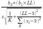
where:
b0 is the intercept of the probability plot's fitted line
b1 is the slope of the probability plot's fitted line
LL is the lower tolerance limit
s is the error standard deviation calculated using the fitted line
K is the number of parts
xi is the reference value of each part
is the mean of the reference values