Weibull and Reliability/Failure Time Analysis - Parameter Estimation
- Maximum likelihood estimation
- STATISTICA computes maximum likelihood parameter estimates for the two- and three-parameter Weibull distribution, with or without censored observations. The specific methods for estimating the parameters are described in Dodson (1994); a detailed description of a Newton-Raphson iterative method, similar to the one used in STATISTICA, for estimating the maximum likelihood parameters for the two-parameter distribution is provided in Keats and Lawrence (1997).
The estimation of the location parameter for the three-parameter Weibull distribution poses a number of special problems, which are detailed in Lawless (1982). Specifically, when the shape parameter is less than 1, then a maximum likelihood solution does not exist for the parameters. In other instances, the likelihood function may contain more than one maximum (i.e., multiple local maxima). In the latter case, Lawless recommends using the smallest failure time (or a value that is a little bit less) as the estimate of the location parameter. In general, STATISTICA follows these recommendations. However, the Results dialog provides interactive options to "experiment" with different parameters (e.g., you may set the location parameter to a particular value, and then compute the maximum likelihood parameter estimates, contingent on this user-defined value of the location parameter); alternative options for estimating parameters are also provided.
- Nonparametric (rank-based) probability plots
- You can derive a descriptive estimate of the cumulative distribution function (regardless of distribution) by first rank-ordering the observations, and then computing any of the following expressions:
- Median rank
-
F(t) = (j-0.3)/(n+0.4)
Mean rank.
F(t) = j/(n+1)
White's plotting position.
F(t) = (j-3/8)/(n+1/4)
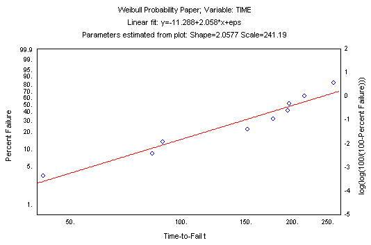
where j denotes the failure order (rank; for multiple-censored data a weighted average ordered failure is computed; see Dodson, p. 21), and n is the total number of observations. You can then construct the following plot.
Note: the horizontal Time-to-fail t axis is scaled logarithmically; on the vertical axis the quantity log(log(100/(100-F(t))) is plotted (a probability scale is shown on the left y-axis). From this plot the parameters of the two-parameter Weibull distribution can be estimated; specifically, the shape parameter is equal to the slope of the linear fit-line, and the scale parameter can be estimated as exp(-intercept/slope). - Estimating the location parameter from probability plots
- It is apparent in the plot shown above that the regression line provides a good fit to the data. When the location parameter is misspecified (e.g., not equal to zero), then the linear fit is worse as compared to the case when it is appropriately specified. Therefore, you can compute the probability plot for several values of the location parameter, and observe the quality of the fit. These computations are summarized in the following plot (accessible from the
Results dialog).
Here the common R-square measure (correlation squared) is used to express the quality of the linear fit in the probability plot, for different values of the location parameter shown on the horizontal x axis (this plot is based on the example data set in Dodson, 1994, Table 2.9). This plot is often very useful when the maximum likelihood estimation procedure for the three-parameter Weibull distribution fails, because it shows whether or not a unique (single) optimum value for the location parameter exists (as in the plot shown above).
Hazard plotting. Another method for estimating the parameters for the two-parameter Weibull distribution is via hazard plotting (as discussed earlier, the hazard function describes the probability of failure during a very small time increment, assuming that no failures have occurred prior to that time). This method is very similar to the probability plotting method. First plot the cumulative hazard function against the logarithm of the survival times; then fit a linear regression line and compute the slope and intercept of that line. As in probability plotting, the shape parameter can then be estimated as the slope of the regression line, and the scale parameter as exp(-intercept/slope). See Dodson (1994) for additional details; see also Weibull CDF, Reliability, and Hazard Functions.
- Method of moments
- This method -- to approximate the moments of the observed distribution by choosing the appropriate parameters for the Weibull distribution -- is also widely described in the literature. In fact, this general method is used for fitting the Johnson curves general non-normal distribution to the data, to compute non-normal process capability indices (see Fitting Distributions by Moments). However, the method is not suited for censored data sets, and is therefore not very useful for the analysis of failure time data.
- Comparing the estimation methods
- Dodson (1994) reports the result of a Monte Carlo simulation study, comparing the different methods of estimation. In general, the maximum likelihood estimates proved to be best for large sample sizes (e.g.,
n>15), while probability plotting and hazard plotting appeared to produce better (more accurate) estimates for smaller samples.
A note of caution regarding maximum likelihood based confidence limits. STATISTICA will compute confidence intervals for maximum likelihood estimates, and for the reliability function based on the standard errors of the maximum likelihood estimates. Dodson (1994) cautions against the interpretation of confidence limits computed from maximum likelihood estimates, or more precisely, estimates that involve the information matrix for the estimated parameters. When the shape parameter is less than 2, the variance estimates computed for maximum likelihood estimates lack accuracy, and it is advisable to compute the various results graphs based on nonparametric confidence limits as well.