Power Analysis and Sample Size Calculation in Experimental Design - Graphical Approaches to Power Analysis
In the preceding discussion, we arrived at a necessary sample size of 607 under the assumption that p is precisely .80. In practice, of course, we would be foolish to perform only one power calculation, based on one hypothetical value. For example, suppose the function relating required sample size to p is particularly steep in this case. It might then be that the sample size required for a p of .70 is much different than that required to reliably detect a p of .80.
Intelligent analysis of power and sample size requires the construction, and careful evaluation, of graphs relating power, sample size, the amount by which the null hypothesis is wrong (i.e., the experimental effect), and other factors such as Type I error rate. Power Analysis allows the convenient construction of a wide range of power and sample size graphs.
In the example discussed in the preceding section, the goal, from the standpoint of the politician, is to plan a study that can decide, with a low probability of error, whether the support level is greater than .50. Graphical analysis can shed a considerable amount of light on the capabilities of a statistical test to provide the desired information under such circumstances.
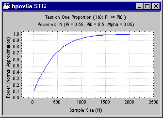
For example, the researcher could plot power against sample size, under the assumption that the true level is .55, i.e., 55%. You might start with a graph that covers a very wide range of sample sizes, to get a general idea of how the statistical test behaves. The following graph shows power as a function of sample sizes ranging from 20 to 2000, using a "normal approximation" to the exact binomial distribution.
The previous graph demonstrates that power reaches an acceptable level (often considered to be between .80 and .90) at a sample size of approximately 600.
Remember, however, that this calculation is based on the supposition that the true value of p is .55. It may be that the shape of the curve relating power and sample size is very sensitive to this value. The question immediately arises, "how sensitive is the slope of this graph to changes in the actual value of p?
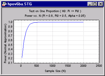
There are a number of ways to address this question. You can plot power vs. sample size for other values of p, for example. Below is a graph of power vs. sample size for p = .6.
You can see immediately in the preceding graph that the improvement in power for increases in N occurs much more rapidly for p = .6 than for p = .55. The difference is striking if you merge the two graphs into one, as shown below:
In planning a study, particularly when a grant proposal must be submitted with a proposed sample size, you must estimate what constitutes a reasonable minimum effect that you wish to detect, a minimum power to detect that effect, and the sample size that will achieve that desired level of power. This sample size can be obtained by analyzing the above graphs, or the Power Analysis module can calculate it directly. For example, if you request the minimum sample size required to achieve a power of .90 when p = .55, Power Analysis can calculate this directly. The result is reported in a spreadsheet, as below:
Results can also be reported in paragraph form suitable for inclusion in a grant proposal. To do so, select the Also send to Report Window check box on the Options - Output Manager tab, select the Display supplementary information check box, and move the slider to Comprehensive. When the results spreadsheet is displayed, they are also sent to the report in paragraph form.
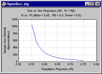
For a given level of power, a graph of sample size vs. p can show how sensitive the required sample size is to the actual value of p. This can be important in gauging how sensitive the estimate of a required sample size is. For example, the following graph shows values of N needed to achieve a power of .90 for various values of p, when the null hypothesis is that p = .50
The preceding graph demonstrates how the required N drops off rapidly as p varies from .55 to .60. To be able to reliably detect a difference of .05 (from the null hypothesized value of .50) requires an N greater than 800, but reliable detection of a difference of .10 requires an N of only around 200. Obviously, then, required sample size is somewhat difficult to pinpoint in this situation. It is much better to be aware of the overall performance of the statistical test against a range of possibilities before beginning an experiment, than to be informed of an unpleasant reality after the fact. For example, imagine that the experimenter had estimated the required sample size on the basis of reliably (with power of .90) detecting a p of .6. The experimenter budgets for a sample size of, say, 220, and imagines that minor departures of p from .6 will not require substantial differences in N. Only later does the experimenter realize that a small change in p requires a huge increase in N , and that the planning for the experiment was optimistic. In some such situations, a "window of opportunity" may close before the sample size can be adjusted upward.
Across a wide variety of analytic situations, power analysis and sample size estimation involve steps that are fundamentally the same:
- The type of analysis and null hypothesis are specified
- Power and required sample size for a reasonable range of effects is investigated.
- The sample size required to detect a reasonable experimental effect (i.e., departure from the null hypothesis), with a reasonable level of power, is calculated, while allowing for a reasonable margin of error.


