Power Analysis and Sample Size Calculation in Experimental Design - Calculating Required Sample Size
To ensure a statistical test will have adequate power, one usually must perform special analyses prior to running the experiment, to calculate how large an N is required.
Let's briefly examine the kind of statistical theory that lies at the foundation of the calculations used to estimate power and sample size. Return to the original example of the politician, contemplating how large an opinion poll should be taken to suit her purposes.
Statistical theory, of course, cannot tell us what will happen with any particular opinion poll. However, through the concept of a sampling distribution, it can tell us what will tend to happen in the long run, over many opinion polls of a particular size.
A sampling distribution is the distribution of a statistic over repeated samples. Consider the sample proportion p resulting from an opinion poll of size N, in the situation where the population proportion π is exactly .50. Sampling distribution theory tells us that p will have a distribution that can be calculated from the binomial theorem. This distribution, for reasonably large N, and for values of π not too close to 0 or 1, looks very much like a normal distribution with a mean of π and a standard deviation (called the "standard error of the proportion") of
σp = sqrt[π(1-π)/N]
Suppose, for example, the politician takes an opinion poll based on an N of 100. Then the distribution of p, over repeated samples, will look like this if π = .5.
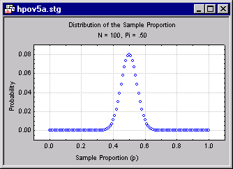
The values are centered around .5, but a small percentage of values are greater than .6 or less than .4. This distribution of values reflects the fact that an opinion poll based on a sample of 100 is an imperfect indicator of the population proportion π.
If p were a "perfect" estimate of π, the standard error of the proportion would be zero, and the sampling distribution would be a spike located at 0.5. The spread of the sampling distribution indicates how much "noise" is mixed in with the "signal" generated by the parameter.
Notice from the equation for the standard error of the proportion that, as N increases, the standard error of the proportion gets smaller. If N becomes large enough, we can be very certain that our estimate p will be a very accurate one.
Suppose the politician uses a decision criterion as follows. If the observed value of p is greater than .58, she will decide that the null hypothesis that π is less than or equal to .50 is false. This rejection rule is diagrammed below.
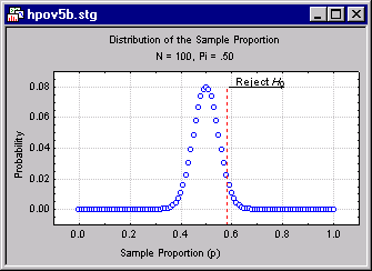
You can, by adding up all the probabilities (computable from the binomial distribution), determine that the probability of rejecting the null hypothesis when π = .50 is .044. Hence, this decision rule controls the Type I Error rate, α, at or below .044. It turns out, this is the lowest decision criterion that maintains α at or below .05.
However, the politician is also concerned about power in this situation, because it is by rejecting the null hypothesis that she is able to support the notion that she has public opinion on her side.
Suppose that 55% of the people support the politician, that is, that π = .55 and the null hypothesis is actually false. In this case, the correct decision is to reject the null hypothesis. What is the probability that she will obtain a sample proportion greater than the "cut-off" value of .58 required to reject the null hypothesis?
In the figure below, we have superimposed the sampling distribution for p when π = .55. Clearly, only a small percentage of the time will the politician reach the correct decision that she has majority support. The probability of obtaining a p greater than .58 is only .241.

Needless to say, there is no point conducting an experiment in which, if your position is correct, it will only be verified 24.1% of the time! In this case a statistician would say that the significance test has "inadequate power to detect a departure of 5 percentage points from the null hypothesized value."
The crux of the problem lies in the width of the two distributions in the preceding figure. If the sample size were larger, the standard error of the proportion would be smaller, and there would be little overlap between the distributions. Then it would be possible to find a decision criterion that provides a low α and high power.
The question is, "How large an N is necessary to produce a power that is reasonably high" in this situation, while maintaining α at a reasonably low value.
You could, of course, go through laborious, repetitive calculations in order to arrive at such a sample size. However, the STATISTICA Power Analysis module performs them automatically, with just a few clicks of the mouse. Moreover, for each analytic situation that it handles, the STATISTICA power module provides extensive capabilities for analyzing, and graphing, the theoretical relationships between power, sample size, and the variables that affect them. The Power Analysis module assumes that you will be employing the well known Chi-square test, rather than the exact binomial test. Suppose that the politician decides that she requires a power of .80 to detect a π of .55. It turns out a sample size of 607 will yield a power of exactly .8009. (The actual Alpha of this test, which has a nominal level of .05, is .0522 in this situation.)