Overview - ANOVA and REML Estimation Methods
The basic goal of variance component estimation is to estimate the population covariation between random factors and the dependent variable. Depending on the method used to estimate variance components, the population variances of the random factors can also be estimated, and significance tests can be performed to test whether the population covariation between the random factors and the dependent variable are nonzero.
Estimating the Variation of Random Factors
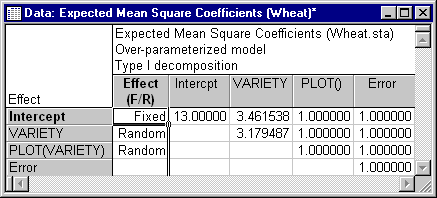
The ANOVA method provides an integrative approach to estimating variance components, because ANOVA techniques can be used to estimate the variance of random factors, to estimate the components of variance in the dependent variable attributable to the random factors, and to test whether the variance components differ significantly from zero. The ANOVA method for estimating the variance of the random factors begins by constructing the Sums of squares and cross products (SSCP) matrix for the independent variables. The sums of squares and cross products for the random effects are then residualized on the fixed effects, leaving the random effects independent of the fixed effects, as required in the mixed model (see, for example, Searle, Casella, & McCulloch, 1992). The residualized Sums of squares and cross products for each random factor are then divided by their degrees of freedom to produce the coefficients in the Expected mean squares matrix. Nonzero off-diagonal coefficients for the random effects in this matrix indicate confounding, which must be taken into account when estimating the population variance for each factor. For the Wheat.sta data, treating both Variety and Plot as random effects, the coefficients in the Expected mean squares matrix show that the two factors are at least somewhat confounded. The Expected mean squares spreadsheet is shown below.
The coefficients in the Expected mean squares matrix are used to estimate the population variation of the random effects by equating their variances to their expected mean squares. For example, the estimated population variance for Variety using Type I Sums of squares would be 3.179487 times the Mean square for Variety plus 1 times the Mean square for Plot plus 1 times the Mean square for Error.
The ANOVA method provides an integrative approach to estimating variance components, but it is not without problems (i.e., ANOVA estimates of variance components are generally biased, and can be negative, even though variances, by definition, must be either zero or positive). In the Variance Estimation and Precision module, an alternative to ANOVA estimation is provided by restricted maximum likelihood estimation (REML).
The REML method is based on quadratic forms and requires iteration to find a solution for the variance components. REML estimation begins by constructing the Quadratic sums of squares (SSQ) matrix. The elements for the random effects in the SSQ matrix can most simply be described as the sums of squares of the sums of squares and cross products for each random effect in the model (after residualization on the fixed effects). The elements of this matrix provide coefficients, similar to the elements of the Expected Mean Squares matrix, which are used to estimate the covariances among the random factors and the dependent variable. The SSQ matrix for the Wheat.sta data is shown below. Note that the nonzero off-diagonal element for Variety and Plot again shows that the two random factors are at least somewhat confounded.
The estimates in this SSQ matrix serve as initial estimates of the covariances among the random factors and the dependent variable.
Estimating Components of Variation
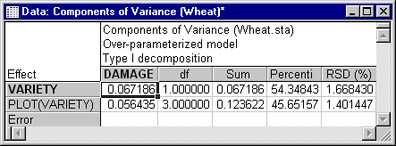
For ANOVA methods for estimating variance components, a solution is found for the system of equations relating the estimated population variances and covariances among the random factors to the estimated population covariances between the random factors and the dependent variable. The solution then defines the variance components. The spreadsheet below shows the Type I Sums of squares estimates of the variance components for the Wheat.sta data.
REML variance components are estimated by iteratively optimizing the parameter estimates for the effects in the model. In REML the likelihood of the data is maximized only for the random effects, thus REML is a restricted maximum likelihood solution. In REML, an iterative solution is found for the weights for the random effects in the model that maximize the likelihood of the data.
The statistical theory underlying maximum likelihood variance component estimation techniques is an advanced topic (Searle, Casella, & McCulloch, 1992, is recommended as an authoritative and comprehensive source). Implementation of maximum likelihood estimation algorithms, furthermore, is difficult (see, for example, Hemmerle & Hartley, 1973, and Jennrich & Sampson, 1976, for descriptions of these algorithms), and faulty implementation can lead to variance component estimates that lie outside the parameter space, converge prematurely to nonoptimal solutions, or give nonsensical results. Milliken and Johnson (1992) noted all of these problems with the commercial software packages they used to estimate variance components. In the Variance Estimation and Precision module, care has been taken to avoid these problems as much as possible. Note, for example, that for the analysis reported in Example 2: Variance Component Estimation for a Four-Way Mixed Factorial Design, most statistical packages do not give reasonable results.
The basic idea behind REML estimation is to find the set of weights for the random effects in the model that minimize the negative of the natural logarithm times the likelihood of the data (the likelihood of the data can vary from zero to one, so minimizing the negative of the natural logarithm times the likelihood of the data amounts to maximizing the probability, or the likelihood, of the data). The REML variance component estimates for the Wheat.sta data are shown below.
As can be seen, the estimates of the Variety variance component for the different methods are quite similar. In general, components of variance using different estimation methods tend to agree fairly well (see, for example, Swallow & Monahan, 1984); however, sometimes differences do occur which may be of practical importance.
Hessian was singular at point of convergence
In some cases (as in the spreadsheet above) you may see this message at the top of the spreadsheet reporting the estimates of the variance components; usually, you will also see at least one component with a reported asymptotic standard error of 0 (zero). This message indicates that during the iterative computations, at least two components were found to be entirely redundant, and that no unique estimates can be derived for those components. This may, for example, happen when there are 0 (zero) degrees of freedom for the error term, and hence, the error variance is not defined.
The computational algorithm used in STATISTICA always attempts to resolve any redundancies so as to retain a positive (>0) estimate for the Error variance component (otherwise, if during the estimation an intermediate solution makes the Error component equal to 0 [zero], the algorithm may prematurely terminate with a non-maximum likelihood solution). However, when this message appears in the header of a results spreadsheet in your analysis, you should carefully review the current model (e.g., click the ANOVA table button on the Variance Estimation and Precision Results dialog - Summary tab), and interpret the estimates of the variance components with caution (as they are not unique).


