Characteristics of Classification Trees - The Power and Pitfalls of Classification Trees
The advantages of classification trees over traditional methods such as linear discriminant analysis, at least in some applications, can be illustrated using a simple, fictitious data set. To keep the presentation even-handed, other situations in which linear discriminant analysis would outperform classification trees are illustrated using a second data set.
Suppose you have records of the Longitude and Latitude coordinates at which 37 storms reached hurricane strength for two classifications of hurricanes - Baro hurricanes and Trop hurricanes. The fictitious data shown below were presented for illustrative purposes by Elsner, Lehmiller, and Kimberlain (1996), who investigated the differences between baroclinic and tropical North Atlantic hurricanes. The data are also available in the example data file Barotrop.sta.
 A linear discriminant analysis of hurricane Class (Baro or Trop) using Longitude and Latitude as predictors correctly classifies only 20 of the 37 hurricanes (54%). A classification tree for Class using the
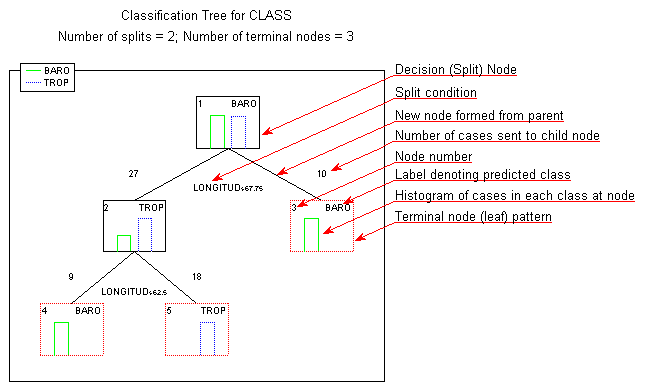
C&RT-style exhaustive search for univariate splits option correctly classifies all 37 hurricanes. The Tree graph for the classification tree is shown below.
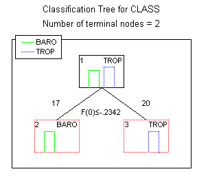
The headings of the graph give the summary information that the classification tree has 2 splits and 3 terminal nodes. Terminal nodes, or terminal leaves as they are sometimes called, are points on the tree beyond which no further decisions are made. In the graph itself, terminal nodes are outlined with dotted red lines, while the remaining decision nodes or split nodes are outlined with solid black lines. The tree starts with the top decision node, sometimes called the root node. In the graph it is labeled as node 1 in its top-left corner. Initially, all 37 hurricanes are assigned to the root node and tentatively classified as Baro hurricanes, as indicated by the Baro label in the top-right corner of the root node. Baro is chosen as the initial classification because there are slightly more Baro than Trop hurricanes, as indicated by the histogram plotted within the root node. The legend identifying which bars in the node histograms correspond to Baro and Trop hurricanes is located in the top-left corner of the graph.
The root node is split, forming two new nodes. The text below the root node describes the split. It indicates that hurricanes with Longitude coordinate values of less than or equal to 67.75 are sent to node number 2 and tentatively classified as Trop hurricanes, and that hurricanes with Longitude coordinate values of greater than 67.75 are assigned to node number 3 and classified as Baro hurricanes. The values of 27 and 10 printed above nodes 2 and 3, respectively, indicate the number of cases sent to each of these two child nodes from their parent, the root node. Similarly, node 2 is subsequently split. The split is such that the 9 hurricanes with Longitude coordinate values of less than or equal to 62.5 are sent to node number 4 and classified as Baro hurricanes, and the remaining 18 hurricanes with Longitude coordinate values of greater than 62.5 are sent to node number 5 and classified as Trop hurricanes.
The tree graph presents all this information in a simple, straightforward way, and probably allows one to digest the information in much less time than it takes to read the two preceding paragraphs. Getting to the bottom line, the histograms plotted within the tree's terminal nodes show that the classification tree classifies the hurricanes perfectly. Each of the terminal nodes is "pure," containing no misclassified hurricanes. All the information in the tree graph is also available in the tree structure spreadsheet shown below.
| Tree Structure (barotrop.sta) | |||||||
| CLASSIF.
TREES |
Child nodes, observed class n's,
predicted class, and split condition for each node |
||||||
| Node | Left
branch |
Right
branch |
n in cls
BARO |
n in cls
TROP |
Predict.
class |
Split
constant |
Split
variable |
| 1
2 3 4 5 |
2
4 |
3
5 |
19
9 10 9 0 |
18
18 0 0 18 |
BARO
TROP BARO BARO TROP |
-67.75
-62.50 |
LONGITUD
LONGITUD |
Note that in the spreadsheet nodes 3 through 5 are identified as terminal nodes because no split is performed at those nodes. Also note the signs of the Split constants displayed in the spreadsheet, for example, -67.75 for the split at node 1. In the tree graph, the split condition at node 1 is described as LONGITUD <= 67.75 rather than as (the equivalent) -67.75 + LONGITUD <= 0. This is done simply to save space on the graph.
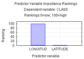
When univariate splits are performed, the predictor variables can be ranked on a 0 - 100 scale in terms of their potential importance in accounting for responses on the dependent variable (see Breiman et al. (1984), pp. 146-150 for details on how these rankings are calculated). For this example, Longitude is clearly very important and Latitude is relatively unimportant.
A classification tree for Class using the discriminant-based univariate split selection method option produces similar results. The tree structure spreadsheet shown for this analysis shows that the splits of -63.4716 and -67.7516 are quite similar to the splits found using the C&RT-style exhaustive search for univariate splits option, although 1 Trop hurricane in terminal node 2 is misclassified as Baro.
| Tree Structure (barotrop.sta) | |||||||
| CLASSIF.
TREES |
Child nodes, observed class n's,
predicted class, and split condition for each node |
||||||
| Node | Left
branch |
Right
branch |
n in cls
BARO |
n in cls
TROP |
Predict.
class |
Split
constant |
Split
variable |
| 1
2 3 4 5 |
2
4 |
3
5 |
19
9 10 0 10 |
18
1 17 17 0 |
BARO
BARO TROP TROP BARO |
-63.4716
-67.7516 |
LONGITUD
LONGITUD |
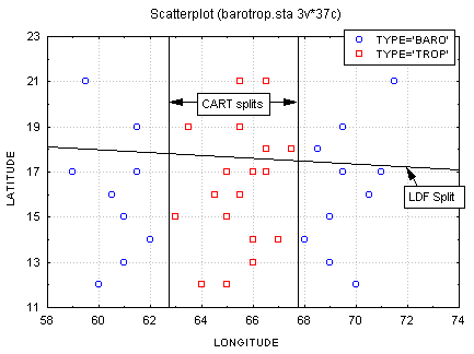
A categorized scatterplot for Longitude and Latitude clearly shows why linear discriminant analysis fails so miserably at predicting Class, and why the classification tree succeeds so well.
The plot clearly shows that there is no strong linear relationship of longitude or latitude coordinates with Class, or of any possible linear combination of longitude and latitude with Class. Class is not functionally related to longitude or latitude, at least in the linear sense. The LDF (Linear Discriminant Function) Split shown on the graph is almost a "shot in the dark" at trying to separate predicted Trop hurricanes (above the split line) from predicted Baro hurricanes (below the split line). The C&RT univariate splits, because they are not restricted to a single linear combination of longitude and latitude scores, find the "cut points" on the Longitude dimension that allow the best possible (in this case, perfect) classification of hurricane Class.
Now we can examine a situation illustrating the pitfalls of classification tree. Suppose that the following hurricane data were available. This data set can be found in the example data file Barotro2.sta.
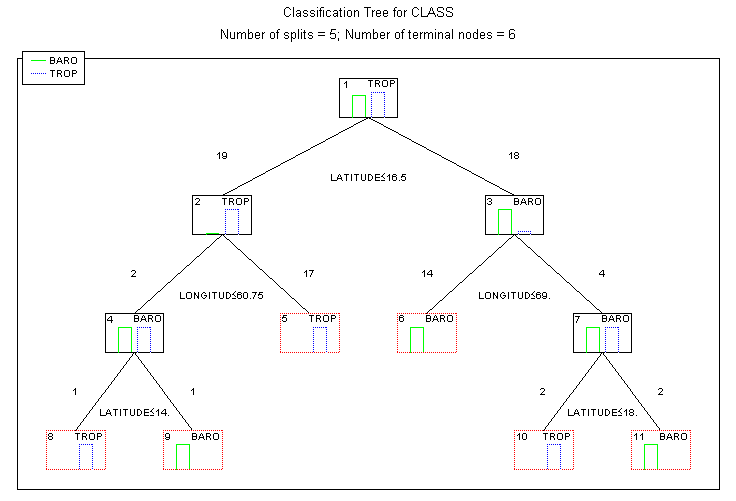
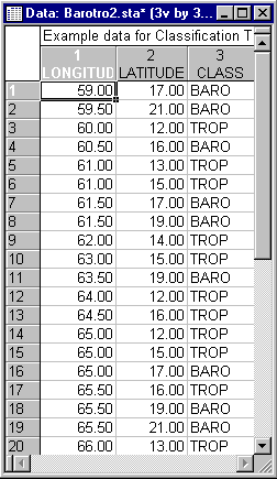 A linear discriminant analysis of hurricane Class (Baro or Trop) using Longitude and Latitude as predictors correctly classifies all 37 of the hurricanes. A classification tree analysis for Class using the C&RT-style exhaustive search for univariate splits option also correctly classifies all 37 hurricanes, but the tree requires 5 splits producing 6 terminal nodes. Which results are easier to interpret? In the linear discriminant analysis, the raw canonical discriminant function coefficients for Longitude and Latitude on the (single) discriminant function are .122073 and -.633124, respectively, and hurricanes with higher longitude and lower latitude coordinates are classified as Trop. The interpretation would be that hurricanes in the western Atlantic at low latitudes are likely to be Trop hurricanes, and that hurricanes further east in the Atlantic at higher latitudes are likely to be Baro hurricanes.
The tree graph for the classification tree analysis using the C&RT-style exhaustive search for univariate splits option is shown below. (To reproduce these results, also select the Fact-style direct stopping option on the Stopping options tab.)
One could methodically describe the splits in this classification tree, exactly as was done in the previous example, but because there are so many splits, the interpretation would necessarily be more complex than the simple interpretation provided by the single discriminant function from the linear discrimination analysis.
However, recall that in describing the flexibility of the Classification Trees module, it was noted that the module has an option for Discriminant-based linear combination splits for ordered predictors using algorithms from QUEST. The tree graph for the classification tree analysis using linear combination splits is shown below.
The moral of this story of the power and pitfalls of classification trees is that classification trees are only as good as the choice of analysis option used to produce them. For finding models that predict well, there is no substitute for a thorough understanding of the nature of the relationships between the predictor and dependent variables.
We have seen that classification trees analysis can be characterized as a hierarchical, highly flexible set of techniques for predicting membership of cases or objects in the classes of a categorical dependent variable from their measurements on one or more predictor variables. With this groundwork behind us, we now are ready to look at the methods for computing classification trees in greater detail.
Techniques and issues in computing classification trees are described in Computational Methods. For information on the basic purpose of classification trees, see the Basic Ideas section of the Introductory Overview.
See also, Exploratory Data Analysis and Data Mining Techniques.

