GLM Introductory Overview - One-Way ANOVA
A design with a single categorical predictor variable is called a one-way ANOVA design. For example, a study of 4 different fertilizers used on different individual plants could be analyzed via one-way ANOVA, with four levels for the factor Fertilizer.
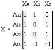
In general, consider a single categorical predictor variable A with 1 case in each of its 3 categories. Using the sigma-restricted coding of A into 2 quantitative contrast variables, the matrix X defining the between design is:
That is, cases in groups A1, A2, and A3 are all assigned values of 1 on X0 (the intercept), the case in group A1 is assigned a value of 1 on X1 and a value 0 on X2, the case in group A2 is assigned a value of 0 on X1 and a value 1 on X2, and the case in group A3 is assigned a value of -1 on X1 and a value -1 on X2. Of course, any additional cases in any of the 3 groups would be coded similarly. If there were 1 case in group A1, 2 cases in group A2, and 1 case in group A3, the X matrix would be:
where the first subscript for A gives the replicate number for the cases in each group. For brevity, replicates usually are not shown when describing ANOVA design matrices.
Using the overparameterized model to represent A, the X matrix defining the between design is simply:
These simple examples show that the X matrix actually serves two purposes. It specifies (1) the coding for the levels of the original predictor variables on the X variables used in the analysis as well as (2) the nature, number, and arrangement of the X variables, that is, the between design.
Between-subject designs
Within-subject (repeated measures) designs
Multivariate designs


