Capability Analysis - Binomial and Poisson - Computational Details
Binomial Case
The Binomial Distribution is described in the Glossary.
This distribution is appropriate for defect data if the proportion of defects per sample is expected to be stable, if all observations have an equal probability of being defective, and if the observations are independent.
Average p (proportion defective), percent defective, PPM
The average p is computed as the total number of defects across all samples divided by the total number of observations across all samples (sum of defects divided by sum of sample sizes).
The percent defective is computed as: 100*p
The observed parts-per-million defective or PPM is computed as 1,000,000*p
For the binomial case, z is computed as normal distribution variate z value corresponding to the normal probability 1-(Average p). This index can be taken as a process capability index, as it reflects on the expected proportion of nonconforming parts (defects).
Upper and Lower Bound Values
Let
D(total) be the total number of defects
N(total) the total number of observations (sum over all samples)
df1=2*D(total)
df2=2*(N(total)- D(total)+1)
df3=2*(D(total)+1)
df4=2*(N(total)- D(total)
F(.p,df1,df2) – is the value of the F distribution corresponding to p, for degrees of freedom = df1 and df2.
The 95% bounds (lower and upper) for the Average p value are:
Lower bound = (df1*F(.025,df1,df2))/(df2+df1* F(.025,df1,df2))
Upper bound = (df3*F(.975,df3,df4))/(df4+df3* F(.975,df3,df4))
Mean defective, Mean DPU
The mean defects per sample are computed as the total number of defects over all samples, divided by the number of samples.
The DPU (defects per unit) estimate is computed as the total number of defects over all samples, divided by the sum of the sample sizes.
Upper and lower Bounds
Let
N(samples) be the number of samples
D(total) be the total number of defects
N(total) the total number of observations (sum over all samples)
df1=2*D(total)
df2=2*(D(total)+1)
ChiSquare(p,df) be the Chi-square value associated with the respective values of p and df
The 95% bounds (lower and upper) for the Mean defective value are:
Lower bound = ChiSquare(.025,df1)/(2*N(samples))
Upper bound = ChiSquare(.975,df2)/(2*N(samples))
The bounds for the mean DPU value (mean defective per Unit) are computed analogously, but dividing the respective ChiSquare Values by 2*N(total).
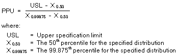
Ppk(ISO)
In addition, Statistica will compute a Binomial or Poisson Process Capability Histogram, which will show a value of process capability, relative to the user-specified upper specification limit.
This value is computed consistent with ISO 21747 M1,l=3,d=6).
Ppk
Statistica will also compute a normal-distribution equivalent Ppk index (see Kotz and Johnson, 2002).
Specifically, the program will compute the respective percentile value associated with the USL value, for the respective fitted (binomial or Poisson) distribution; this value is then converted into a normal distribution z value, and divided by 3.