Support Vector Machines Introductory Overview
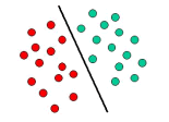
Support Vector Machines are based on the concept of decision planes that define decision boundaries. A decision plane is one that separates between a set of objects having different class memberships. A schematic example is shown in the illustration below. In this example, the objects belong either to class GREEN or RED. The separating line defines a boundary on the right side of which all objects are GREEN and to the left of which all objects are RED. Any new object (white circle) falling to the right is labeled, i.e., classified, as GREEN (or classified as RED should it fall to the left of the separating line).

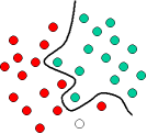
The above is a classic example of a linear classifier, i.e., a classifier that separates a set of objects into their respective groups (GREEN and RED in this case) with a line. Most classification tasks, however, are not that simple, and often more complex structures are needed in order to make an optimal separation, i.e., correctly classify new objects (test cases) on the basis of the examples that are available (train cases). This situation is depicted in the illustration below. Compared to the previous schematic, it is clear that a full separation of the GREEN and RED objects would require a curve (which is more complex than a line). Classification tasks based on drawing separating lines to distinguish between objects of different class memberships are known as hyperplane classifiers. Support Vector Machines are particularly suited to handle such tasks.

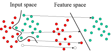
The illustration below shows the basic idea behind Support Vector Machines. Here we see the original objects (left side of the schematic) mapped, i.e., rearranged, using a set of mathematical functions, known as kernels. The process of rearranging the objects is known as mapping (transformation). Note that in this new setting, the mapped objects (right side of the schematic) are linearly separable and, thus, instead of constructing the complex curve (left schematic), all we have to do is to find an optimal line that can separate the GREEN and the RED objects.

Technical Notes
STATISTICA Support Vector Machine (SVM) is primarily a classier method that performs classification tasks by constructing hyperplanes in a multidimensional space that separates cases of different class labels. STATISTICA SVM supports both regression and classification tasks and can handle multiple continuous and categorical variables. For categorical variables a dummy variable is created with case values as either 0 or 1. Thus, a categorical dependent variable consisting of three levels, say (A, B, C), is represented by a set of three dummy variables:
A: {1 0 0}, B: {0 1 0}, C: {0 0 1}
To construct an optimal hyperplane, SVM employs an iterative training algorithm, which is used to minimize an error function. According to the form of the error function, SVM models can be classified into four distinct groups:
- Classification SVM Type 1 (also known as C-SVM classification)
- Classification SVM Type 2 (also known as nu-SVM classification)
- Regression SVM Type 1 (also known as epsilon-SVM regression)
- Regression SVM Type 2 (also known as nu-SVM regression)
Following is a brief summary of each model.
Classification SVM
Classification SVM Type 1
For this type of SVM, training involves the minimization of the error function:
subject to the constraints:
where C is the capacity constant, w is the vector of coefficients, b is a constant, and ![]() represents parameters for handling nonseparable data (inputs). The index i labels the N training cases. Note that
represents parameters for handling nonseparable data (inputs). The index i labels the N training cases. Note that ![]() represents the class labels and xi represents the independent variables. The kernel
represents the class labels and xi represents the independent variables. The kernel ![]() is used to transform data from the input (independent) to the feature space. It should be noted that the larger the C, the more the error is penalized. Thus, C should be chosen with care to avoid over fitting.
is used to transform data from the input (independent) to the feature space. It should be noted that the larger the C, the more the error is penalized. Thus, C should be chosen with care to avoid over fitting.
Classification SVM Type 2
In contrast to Classification SVM Type 1, the Classification SVM Type 2 model minimizes the error function:
subject to the constraints:
Regression SVM
In a regression SVM, you have to estimate the functional dependence of the dependent variable y on a set of independent variables x. It assumes, like other regression problems, that the relationship between the independent and dependent variables is given by a deterministic function f plus the addition of some additive noise:
y = f (x) + noise
The task is then to find a functional form for f that can correctly predict new cases that the SVM has not been presented with before. This can be achieved by training the SVM model on a sample set, i.e., training set, a process that involves, like classification (see above), the sequential optimization of an error function. Depending on the definition of this error function, two types of SVM models can be recognized:
Regression SVM Type 1
For this type of SVM the error function is:
which we minimize subject to:

Regression SVM Type 2
For this SVM model, the error function is given by:
which we minimize subject to:

Kernel Functions
STATISTICA SVM supports a number of kernels for use in Support Vector Machines models. These include linear, polynomial, radial basis function (RBF), and sigmoid:

| where |
that is, the kernel function, represents a dot product of input data points mapped into the higher dimensional feature space by transformation ![]() .
.
Gamma is an adjustable parameter of certain kernel functions.
The RBF is by far the most popular choice of kernel types used in Support Vector Machines. This is mainly because of their localized and finite responses across the entire range of the real x-axis.
