Stepwise Model Builder - Logistic Regression
Ribbon bar. In Statistica, open a data set. Then, select the Statistics tab. In the Advanced/Multivariate group, click Advanced Models, and select Stepwise Model Builder to display the Stepwise Model Builder - Logistic Regression Startup Panel.
Classic menus. Open a data set. On the Statistics - Advanced Linear/Nonlinear Models submenu, select Stepwise Model Builder to display the Stepwise Model Builder - Logistic Regression Startup Panel.
Overview and Workflow
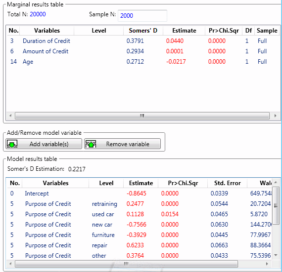
Use the options in the Stepwise Model Builder - Logistic Regression Startup Panel to compute the marginal predictor statistics given a current model; specifically, the variables listed in the Marginal Results Table will be entered one at a time into the logistic regression containing the predictors listed in the Model Results Table, so that analysts can evaluate the unique contribution of each predictor candidate not in the equation.
- Variable/predictor selection, coding
- First, select the variables for the analyses; select a binary (for example, 0/1) dependent or Y variable, and select the two integer values or codes for the Bad code and Good code.
Note: the model will be estimated after recoding all Bad code values to 1 and Good code values to 0.
Then, select two or more continuous or categorical (discrete) predictor candidates (X variables).
Next, select (highlight) the predictor candidates in the Marginal Analysis Variables pane, and click either the Full sample button or the Subsample button to compute the Marginal results table results.
Then select (highlight) the predictors in the Marginal Results Table that are to be entered into the full Model Results Table, and click the Add variable button to:
1) Estimate the parameters of the logistic regression model including the selected predictors and any predictors previously entered into the regression equation, and
2) Re-estimate the results for all predictor candidates in the Marginal Results Table
Estimates from Subsample, Full sample. You can estimate the marginal analysis results (including those accessible via the options in the Marginal Results group box) using either a subsample of observations or all observations; you can also select (highlight) one or more predictors in the Marginal Results Table and re-estimate the respective marginal results for the Full sample or Subsample. The Sample column in the Marginal Results Table indicates whether the currently displayed results were computed from a random Subsample or the Full sample. When the results in the Marginal Results Table are re-estimated after you choose to Add variable or Remove variable from the Model Results Table, the same sample and sample option is used as before (Subsample or Full sample; note that a new Subsample is drawn only when the Subsample button is clicked).
The Model Results Table statistics are always computed for the entire data set.
- Categorical (discrete) predictors
- When the model includes categorical (discrete) predictors, Statistica will use the overparameterized model to code the respective discrete values for those predictors, and then estimate separate parameter estimates for each discrete value, assuming that the respective predictor would be entered "as a whole" into the equation, that is, with all discrete values that it contains.
This means that you cannot separate the set of discrete values available in a discrete predictor candidate, and all values will always be added or removed from models and selections in unison, even if only a single code is selected (highlighted) when the respective predictor is moved in/out of a results table.
When discrete predictors are removed from the prediction equation or the Marginal Results Table, the same logic applies.
- Saving a project (in progress)
- You can save a work-in-progress by clicking the Save project button located in the Project group box, and retrieve it later to continue work by clicking the Open project button. Note that after opening a previously saved project, the next time any results statistics or re-calculations are requested via the options in Stepwise Model Builder, the program will recompute all results necessary to enable you to resume the interactive model building. When working with large projects involving many predictors, this may require some time.
- Validation of model results; bootstrapping
- There are two ways for analysts to assess the robustness of the parameter estimates and results in the Model Results Table. First, results can be computed for a Validation sample. To do so, specify a Validation Sample variable and a Code (in the Validation Sample box at the top-center of the Startup Panel); only cases with this Code value will be used when computing results via the Validation option in the Model Analysis box. Second, the Bootstrap option can be used to estimate parameter values and results statistics for repeatedly drawn samples.
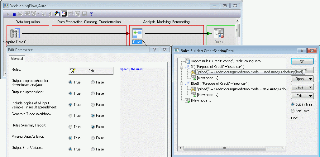
Deploying models to Enterprise, Decisioning Flows. Click the Deploy model button (in the Model group box at the top-right of the Startup Panel) to save models to Enterprise. These models can then be referenced in Decisioning Flows for scoring or conditional scoring using the Rules node.
Option Descriptions
Select variables. Click this button to display a standard variable selection dialog box. Select a discrete (categorical) Dependent or Y variable with at least two codes (binary, for example, credit default), and two or more Continuous and/or Categorical Predictors (predictor candidates). After exiting the variable selection dialog box (click the OK button), the respective variable names will be transferred into the Marginal Analysis Variables pane.
Marginal Analysis Variables. After selecting variables for the analyses, this pane will show the selected variable names, their type (Continuous or Categorical), and the variable number in the input file. You can select one or more predictors in this list by highlighting them; to run marginal analyses on the selected variables, click either the Full sample or Subsample button in the Run Marginal Analysis group box.
Set Logistic Parameters.
- Model parameters
- Click this button to display the
Logistic Regression Model Parameters dialog box, which contains options for parameterization and estimation.
Validation Sample. Optionally, you can select a variable containing codes to identify a validation sample; double-click the top box to display a variable selection dialog box displaying the variables for the analysis. Then, select a Code that identifies the observations that are to be held out for the validation sample, that is, from which to recompute the model analysis results when using the Validation option (button located in the Model Analysis group box). Note that the Validation button will always display the recomputed (from the validation sample) results in results spreadsheets; the results shown in the Model Results Table displayed in the Stepwise Model Builder are always computed for all cases.
Dependent (Y) Variable. As described in the Introductory Overview, the program will compute parameter estimates and other results for a logistic regression. Select here the two (binary) codes that are to be used for the analyses, for the dependent or Y variable.
Note: for the logistic regression analysis, the values specified as Bad codes will be recoded to 1, and the values specified as Good will be recoded to 0.Project. Use the Save project and Open project options to save work in progress and to retrieve previously saved projects to continue working with the same variables and model.
- Open project
- Click this button to display the Open dialog box, which is used to browse to and select a previously saved project. Note that after opening a previously saved project, the next time any results statistics or re-calculations are requested via the options in Stepwise Model Builder, the program will recompute all results necessary to enable you to resume the interactive model building. When working with large projects involving many predictors, this may require some time.
- Save project
- Click this button to display the Save As dialog box, where you can enter a name and specify a location for the project.
Model.
- Deploy model
- Click this button to save the current logistic regression model (equation) to Statistica Enterprise; models saved in Enterprise can be referenced by Enterprise analysis templates, as well as from Rules nodes in decisioning flows. This button is not available until a model is available in the Model Results Table.
- Show Model
- Click this button to output the current logistic regression model to a workbook. This button is dimmed until a model is available in the Model Results Table.
Run Marginal Analysis. Click either the Full sample or Subsample button to add the selected (highlighted) predictor candidates from the Marginal Analysis Variables pane to the Marginal Results Table, and to compute the respective marginal analysis results.
- Full sample
- To estimate the marginal analysis results for the full sample, click this button.
- Subsample
- To estimate the marginal analysis results from a subsample of observations, click the Subsample button; a sample of the size as specified in the Sample N field will be drawn prior to the computation of marginal results statistics.
- Remove variable
- Select a variable in the Marginal Results Table, and click this button to remove the variable and return it to the Marginal Analysis Variables pane.
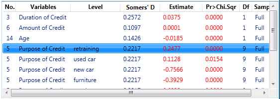
Marginal Results Table. The Marginal Results Table will display the marginal analysis results for the currently selected predictor candidates. Right-click any column header in the Marginal Results Table to display a shortcut menu containing check boxes adjacent to available statistics; when a check box is selected, the respective column is added to the table; when a check box is cleared, the respective column is hidden in the table.
- Total N
- This field displays the number of all observations.
- Sample N
- The entry in this user-specified field determines the approximate sample size that is used to compute Subsample results. Note that the Sample N must be set to at least 500. If a validation sample has been selected, the subsample for the analysis will be chosen from the sample of original data that excludes the validation sample. In the case where there are not enough cases to produce the user requested sample size after excluding the validation sample, the entire analysis sample will be used.
- No
- This column displays the variable numbers of the respective predictors in the input data.
- Variables
- This column displays the names of the predictors in the input data.
- Level
- The values (codes) displayed in this column show the respective discrete values (categories) for categorical predictor candidates. Note that the program will use the overparameterized model, so different parameter estimates are computed for each category. However, the categories of categorical variables can only be deselected/selected from/to the analyses in unison, that is, they cannot be separated, and the other results statistics (Somers' D, p) will be identical for all levels.
- Somers' D/Estimate/Pr>Chi.Sqr.
- These columns display the results statistics.
- Df
- Degrees of freedom for Wald statistic.
- Sample
- This column indicates whether the respective marginal results were computed and will be recomputed by default from either a Subsample of cases or the Full sample (all observations). Note that the user-specified Sample N determines the approximate sample size that is used to compute Subsample results.
Notes:
Sorting the variable list. Click the columns in the Marginal Results Table to sort the table by the respective column values in ascending or descending order.
Selecting predictor candidates in the Marginal Results Table. To select predictor candidates in the Marginal Results Table, click the respective predictor candidate. Use CTRL+click or SHIFT+click to select specific predictor candidates or lists of contiguous predictor candidates, respectively.
Re-calculating marginal results. Click the Full sample or Subsample button to recalculate the marginal analysis results for the highlighted (selected) predictor variables.
Adding variables to the Model Results Table. Click the Add variable button to move selected (highlighted) predictors into the model and to update the Marginal Results Table.
Marginal Results.
- Correlations
- Click the Correlations button to review the correlation of parameter estimates for each predictor candidate in the Marginal Results Table and the parameters in the current Model Results Table.
- Marginal analysis
- Click the Marginal analysis button to review complete parameter estimation table for the model after entering each predictor candidate into the model one by one. Results will be displayed in standard results spreadsheets and graphs, shown by default in workbooks.
Add/Remove Model Variables.
- Add variable
- Click this button to add selected (highlighted) predictor candidates from the Marginal Results Table to the Model Results Table (into the final model). Note that multiple degree-of-freedom effects associated with categorical (discrete) predictor candidates are moved into the model in unison, even if only a single category or value for the respective predictor candidate is highlighted in the Marginal Results Table.
The results in the Model Results Table are always computed for the full sample. After the model parameters are updated, the Marginal Results Table results are then recalculated for all predictor candidates currently not in the model.
- Remove variable
- Click this button to remove selected (highlighted) predictors from the Model Results Table and move them back into the Marginal Results Table.
- Comment for Add/Remove
- Optionally type comments concerning variables added or removed. These comments will be displayed in a column in the Model Building Summary output spreadsheet.
Model Results Table. The Model Results Table shows the parameter estimates and summary statistics for the current model, that is, the model with the predictors listed in the pane and computed from the full sample. Right-click any column header in the Model Results Table to display a shortcut menu containing check boxes adjacent to available statistics; when a check box is selected, the respective column is added to the table; when a check box is cleared, the respective column is hidden in the table.
Note:
Removing variables. To remove predictors from the current model, highlight the respective predictors and then click the Remove variable button. The predictors will be removed from the model, the model will be re-estimated with the remaining predictors, and the Marginal Results Table will be recalculated for all predictor candidates including those that were removed from the model.
Model Analysis.
- Graphs
- Click the Graphs button to compute various diagnostic and residual statistics graphs, including:
- A lift chart for the prediction of the dependent (Y) variable
- Normal probability plot of residuals
- ROC curve and values/statistics
These results are always computed for the current model (with predictors listed in the Model Results Table) and the full sample.
- Validation
- Click this button to compute the Validation results. This button is not available if a Validation Sample has not been specified. First, specify a Validation Sample variable and a Code (see option descriptions above); the data will be divided into a Training and Testing sample based on the selected code. The parameters of the currently specified model will be estimated with those cases in the Training set only, and the model will be deployed on both sets. The following results are generated for both the training and testing data sets for comparison: ROC curve, Lift Chart, Misclassification matrix, and Model comparison statistics, which include Accuracy Ratio, Gini coefficient, Area Under Curve (AUC), Kolmogorov-Smirnov (KS) statistic and p-value, and Hosmer-Lemeshow (HL) Goodness of Fit test statistic and p-value.
- Bootstrap
- Click this button to compute bootstrap error estimates (distributions) for the parameters and for the observed and estimated percent (rate) of 1s (for example, default rates).
Note: the following three options pertain only to Bootstrapping and are not applicable for Graphs or Validation. Specify:
k replications. The number of bootstrap replications
p% in holdout sample. The proportion of hold-out cases for estimating predictive accuracy [and the predicted percent-1s (default rate), as well as the difference between the predicted and observed percent-1s] in the holdout sample in each bootstrap replication; if this value is 0 (zero), predictive accuracy is computed from the (100%) training sample (used for estimating the parameters)
The program will then create k replications of the data via random sampling with replacement, and designate a proportion p cases in each replication as the hold-out or testing sample. Next, the respective model will be fit to all cases not in the hold-out sample (in the training sample) in the respective replication. The parameter estimates and percent (rate) of 1s (for example, percent Default) observed and predicted in the hold-out sample in each replication are also recorded. Thus, you can then evaluate the distribution of the parameter estimates and percent-of-1s observed and predicted over the replications.
If no hold-out sample is designated (Proportion of cases for holdout (p)=0), the respective percent-of-1s observed and predicted will always be computed from the training sample, that is, from all observations in each of the k replications.
Cut-off probability for classification p. Several results graphs, as well as the Bootstrap option, will compute predicted classifications based on prediction probabilities computed by the model. This parameter determines the cut-off probability for classifying a case as 1 (Bad code); that is, if the predicted probability of Bad for an observation is greater than p specified here, the respective observation will be classified as 1 or Bad.
Model Results. Use these options to compute various model statistics and summaries for the current model with predictors listed in the Model Results Table, and computed from the full sample.
- Covariances
- Click this button to produce a covariance matrix of the parameter estimates.
- Correlations
- Click this button to produce a correlation matrix of the parameter estimates.
- Summary
- Click this button to produce several results tables describing the current model, including tables with summary tests for each effect (predictor) in the model and parameter estimates and standard errors, confidence intervals.


