SANN Overviews - Network Types
The Multilayer Perceptron Neural Networks

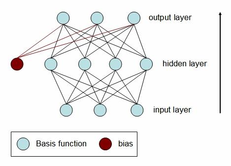
A schematic diagram of a fully connected MLP2 neural network with three inputs, four hidden units (neurons), and three outputs. Note that the hidden and output layers have a bias term. Bias is a neuron that emits a signal with strength 1.
Multilayer perceptrons (MLP) is perhaps the most popular network architecture in use today, due originally to Rumelhart and McClelland (1986) and discussed at length in most neural network textbooks (Bishop, 1995). Each neuron performs a weighted sum of its inputs and passes it through a transfer function f to produce their output. For each neural layer in an MLP network, there is also a bias term. A bias is a neuron in which its activation function is permanently set to 1. Just as like other neurons, a bias connects to the neurons in the layer above via a weight, which is often called threshold. The neurons and biases are arranged in a layered feedforward topology. The network thus has a simple interpretation as a form of input-output model, with the weights and thresholds as the free (adjustable) parameters of the model. Such networks can model functions of almost arbitrary complexity with the number of layers and the number of units in each layer determining the function complexity. Important issues in Multilayer Perceptrons design include specification of the number of hidden layers and the number of units in these layers (Bishop, 1995). Others include the choice of activation functions and methods of training.
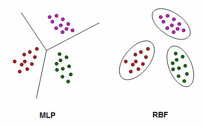
Schematic showing the difference between MLP and RBF neural networks in two-dimensional input data. One way to separate the clusters of inputs is to draw appropriate planes separating the various classes from one another. This method is used by MLP networks. An alternative approach is to fit each class of input data with a Gaussian basis function.
The Radial Basis Function Neural Networks
A schematic diagram of an RBF neural network with three inputs, four radial basis functions and 3 outputs. Note that, in contrast to MLP networks, it is only the output units that have a bias term.
Another type of neural network architecture used by STATISTICA Automated Neural Network is known as Radial Basis Functions (RBF). RBF networks are perhaps the most popular type of neural networks after MLPs. In many ways RBF is similar to MLP networks. First, they too have unidirectional feedforward connections and every neurons is fully connected to the units in the next layer above. The neurons are arranged in a layered feedforward topology. Nonetheless, RBF neural networks models are fundamentally different in the way they model the input-target relationship. While MLP networks model the input-target relationship in one stage, an RBF network partitions this learning process into two distinct and independent stages. In the first stage, and with the aid of the hidden layer neurons known as radial basis functions, the RBF networks model the probability distribution of the input data. In the second stage, RBF learns how to relate an input data x to a target variable t. Note that unlike MLP networks, the bias term of an RBF neural network connects to the output neurons only. In other words, RBF networks do not have a bias term connecting the inputs to the radial basis units. In the following overviews, we will refer to both weights and thresholds as weights unless it is necessary to make a distinction.
Just as with MLP, the activation function of the inputs is taken to be the identity. The signals from these inputs are passed to each radial basis unit in the hidden layer and the Euclidean distance between the input and a prototype vector is calculated for each neuron. This prototype vector is taken to be the location of the basis function in the space of the input data. Each neuron in the output layer performs a weighted sum of its inputs and passes it through a transfer function to produce their output. This means that, unlike an MLP, RBF networks have two types of parameters, (1) the location and radial spread of the basis functions and (2) weights that connect these basis functions to the output units.