Decision Tree Use Case
This use case model demonstrates using a decision tree model to assess the characteristics of the client that leads to the purchase of a new product targeted in a direct marketing campaign.
- Datasets
- In this case, the dependent variable is
y
column of whether the client that was called during a direct marketing campaign subscribed to a term deposit (yes or
no). This dataset comes from the UC Irvine site (http://archive.ics.uci.edu/ml/machine-learning-databases/00222/), and the exact version used for this case is
bank_marketing_data.csv (3.7MB).
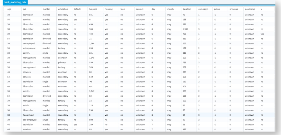
The dataset contains 45,211 observations and 17 columns (16 attributes and 1 dependent value). The attributes analyzed includes the client's age, job type, marital status, education, account default status, housing loan status, personal loan status, contact type, last contact day, last contact month, last contact duration (seconds), # of contacts, # of days since contacted, # of days passed since last contact, previous number of contacts, outcome of previous campaign.
The first few rows are shown below, with y as the dependent variable:
Workflow
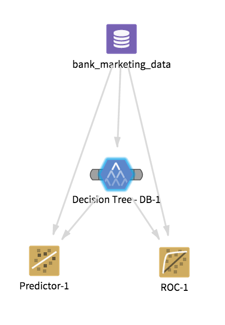
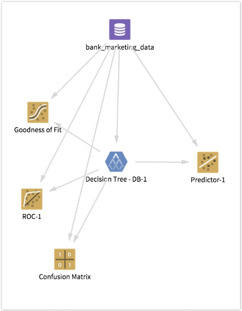
The overall configuration for this Analytic Flow might be something like the following:
For purposes of this example, assume the modeler is trying to understand the question, "Which sub-group of clients should be targeted for the highest subscription rate of a term deposit product?"
If the modeler selects all the variables as independent variables, the results are quite complicated, repetitive and do not seem to reveal any immediate business insights.

In this particular example, the variable month is exploding the Decision Tree and not seeming to add much business decision value.
One approach for avoiding such over-fitting might be to test some initial assumptions the modeler might have regarding the independent variables.
For example, perhaps different clients are more likely to subscribe to a term deposit if they have been well informed on the product during the campaign (got a long enough contact), or already subscribed in the past after a successful marketing campaign.
With this hypothesis in mind, the modeler might reduce the potential independent variables analyzed and select only the contact, duration, campaign, pdays, previous, poutcome variables to include in the analysis. The overall Decision Tree Operator configuration properties can be kept at their default values.
Results
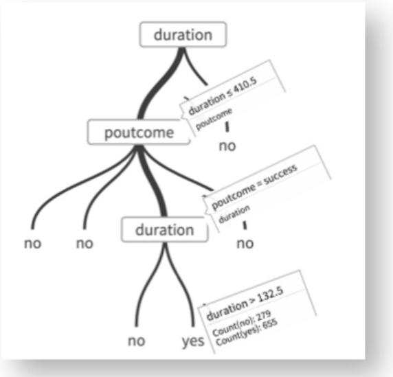
The results in this case are more understandable, revealing the insight that clients for whom the last campaign was successful AND for whom the last call was between 132 and 410 seconds seem to be more likely to subscribe to the term deposit product.
Including the Predictor Operator provides additional model results:
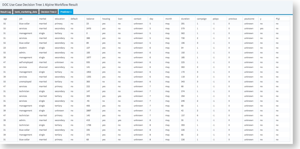
The prediction P(y) value (yes or no) uses a threshold assumption of greater than 50% confidence that the prediction will happen.
Hooking in additional model diagnostic tools, such as the ROC graph, Confusion Matrix, and Goodness Of Fit Operators, provides additional feedback on the quality of the model.
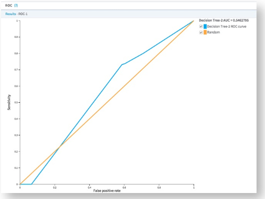
The ROC (Receiver Operating Characteristic) Curve plots the sensitivity (% of correctly classified results) vs. false positives. The larger the AUC value, the more predictive the model is. Any AUC value over .80 is typically considered a "good" model. A value of .5 just means the model is no better than a "dumb" model that can guess the right answer half of the time.
The Goodness of Fit Operator provides model accuracy, error and other validation data.

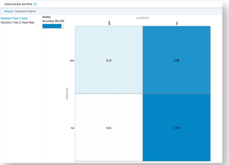
The following confusion matrix table summarizes model accuracy data, and the heat map visual summarizes the actual versus predicted counts of a classification model. These two summaries help assess the model's accuracy for each of the possible class values in a visually intuitive manner.

