Probability Calculation Using Logistic Regression

Team Studio supports the following two common forms of Logistic Regression:

General Principles

Logistic regression analysis predicts the odds of an outcome of a categorical variable based on one or more predictor variables. A categorical variable is one that can take on a limited number of values, levels, or categories, such as "valid" or "invalid". A major advantage of Logistic Regression is its predictions are always between 0 and 1, unlike Linear Regression.

For example, a logistic model might predict the likelihood of a given person going to the beach as a function of temperature. A reasonable model might predict, for example, that a change in 10 degrees makes a person two times more or less likely to go to the beach. The term "twice as likely" for probability refers to the odds doubling (as opposed to the probability doubling). Rather, it is the odds that are doubling: from 2:1 odds, to 4:1 odds, to 8:1 odds, etc. Such a logistic model is called a log-odds model.

Hence, in statistics, Logistic Regression is sometimes called the logistic model or logit model. It is used for predicting the probability of the occurrence of a specific event by fitting data to a logit Logistic Function curve.

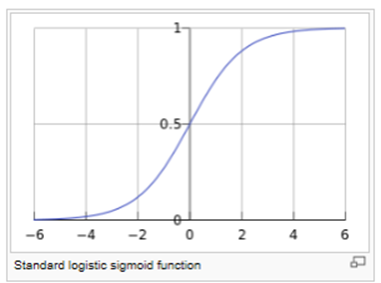
A Logistics Function is represented by an s-curve which was introduced by Pierre Verhulst in 1844, studied in relation to population growth. A generalized logistic curve can model the "S-shaped" behavior (abbreviated S-curve) of growth of some population P. The initial stage of growth is approximately exponential; then, as saturation begins, the growth slows, and at maturity, growth stops. This simple logistic function may be defined by the formula

where the variable P denotes a population, e is Euler's number (2.72), and the variable t might be thought of as time.

http://en.wikipedia.org/wiki/Logistic_function#cite_note-0

For values of X in the range of real numbers from −∞ to +∞, the S-curve shown is obtained. In practice, due to the nature of the exponential functione^−t, it is sufficient to compute t over a small range of real numbers such as [−6, +6].

The following is an example of an S-Curve or Logistic Function.

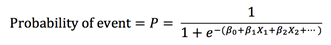
The Logistic Function can be applied to more generalized models that attempt to predict the probability of a specific event. In this case, there may be several factors or variables that contribute to whether the event happens. This Logistic Regression formula can be written generally in a linear equation form as:

Where P = Probability of Event, and are the regression coefficients and X1,X2,… are the independent variable values. Solving for the Probability equation results in:

Logistic Regression Odds Ratio

The odds of an event occurring are defined as the probability of a case divided by the probability of a non-case given the value of the independent variable. The odds ratio is the primary measure of effect size in logistic regression and is computed to compare the odds that membership in one group leads to a case outcome with the odds that membership in some other group leads to a case outcome. The odds ratio (denoted OR) is simply calculated by the odds of being a case for one group divided by the odds of being a case for another group. This calculates how much a change in the independent variable affects the value of the dependent.

As an example, suppose we only know a person's height and we want to predict whether that person is male or female. We can talk about the probability of being male or female, or we can talk about the odds of being male or female. Let's say that the probability of being male at a given height is .90. Then the odds of being male would be:

= .9/.1 = 9 to 1 odds

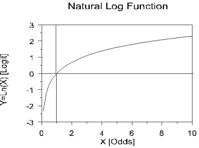
Logistic Regression takes the natural logarithm of the odds (referred to as the logit or log-odds) to create a continuous criterion. The natural log function curve might look like the following.

The logit of success is then fit to the predictors using linear regression analysis. The results of the logit, however, are not intuitive, so the logit is converted back to the odds using the exponential function or the inverse of the natural logarithm. Therefore, although the observed variables in logistic regression are categorical, the predicted scores are actually modeled as a continuous variable (the logit).

Binomial vs. Multinomial Regression

Logistic regression can be binomial or multinomial.

• Binomial or binary logistic regression refers to the instance in which the criterion can take on only two possible outcomes (e.g., "dead" vs. "alive", "success" vs. "failure", or "yes" vs. "no").
  • Note: The Alpine Logistics Regression Operator applies a binomial regression by assuming the dependent variable is either the Value to Predict or Not(Value to Predict).
• Multinomial Logistic Regression (MLOR) refers to the instance in which the criterion can take on three or more possible outcomes (for example, "better' vs. "no change" vs. "worse"). Generally, the criterion is coded as "0" and "1" in binary logistic regression as it leads to the most straightforward interpretation.

Iteratively Reweighted Least Squares (IRLS)

The Alpine Logistic Regression Operator utilizes the method of Iteratively Reweighted Least Squares (IRLS) for calculating the best fitting, etc. Coefficient values. IRLS is a modeling fit optimization method that calculates quantities of statistical interest using weighted least squares calculations iteratively. The process starts off by finding the value of coefficients using the input, observed dataset with a standard least squares estimating approach, just as in Linear Regression modeling. It then takes the first estimate of coefficients and uses them to weight and recalculate the input data (using a mathematical weighting expression). This iterative, re-weighting of the input data continues until convergence is obtained, as defined by the Epsilon.

This IRLS method outputs both coefficients for each variable in the model as well as weights for each observation that help the modeler understand behavior of the algorithm during the iterations. These weights are useful diagnostics for identifying unusual data once convergence has been reached.

The Logistic Regression algorithm uses the Maximum Likelihood (ML) method for finding the smallest possible deviance between the observed and predicted values using calculus derivative calculations. After several iterations, it gets to the smallest possible deviance or best fit. Once it has found the best solution, it provides the final chi-square value for the deviance which is also referred to as the -2LL.

Alternative Models

• Naive Bayes
• Classification Modeling with Decision Tree
• Alpine Forest Classification
• SVM Classification